20230616 Learning to simulate

One of the papers that I like the most on this journey of getting nets to simulate stuff is this one. The results are kinda cool but more importantly the code and data is available. I tried for many hours but could not get the code to run on the gpu. Too many tensorflow and driver compatibility problems as the code used an old version of tensorflow. Not a problem. I shall simply reimplement it myself in pytorch. Something something education!

Exploring the dataset

I first downloaded the WaterDrop dataset. It’s a could of gigs. Let’s take a look at the statistics of the particle positions, vels, and accelerations for a single example: 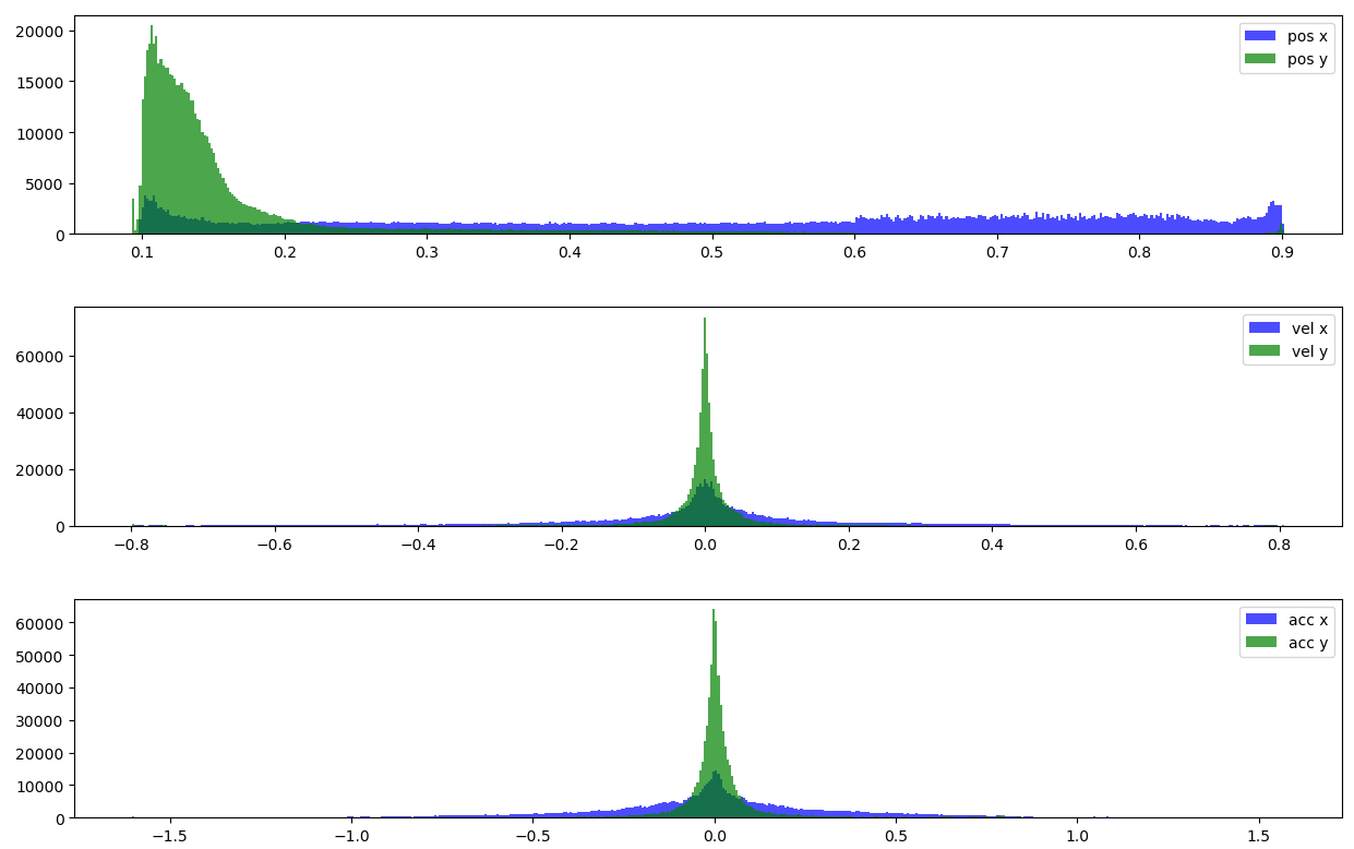Compare this to the statistics here and it actually looks basically the same. Maybe the n body problem is actually pretty representative after all…

Single trajectory

As a first order of business let’s train a model on a single trajectory with the simplest possible model:

class WaterManual(torch.nn.Module):
 
    def __init__(self, num_features: int):
        super().__init__()
        self.hidden_size = int(num_features * 2)
        self.input_conv = Linear(num_features, self.hidden_size)
 
        self.hidden_conv1 = Linear(self.hidden_size, self.hidden_size)
        self.hidden_conv2 = Linear(self.hidden_size, self.hidden_size)
        self.output_conv = Linear(self.hidden_size, num_features) 
 
        # pytorch leaky rely activation:
        self.act = LeakyReLU()
 
 
    def forward(self, x):
        if x.ndim == 2:
            x = x.unsqueeze(0) # batch size 1
        orig_shape = x.shape
 
        x = x.reshape([x.shape[0], -1])   # Flatten input features
 
        x = self.input_conv(x)
        x = self.act(self.hidden_conv1(x))
        x = self.act(self.hidden_conv2(x))
        x = self.output_conv(x)
 
        x = x.reshape(orig_shape)
        return x.squeeze()

A basic MLP with two hidden layers. The examples in the dataset all have different sizes but this isn’t a problem for this contrived and overfit example.

Training

Here is the result of training on a single trajectory with two hidden layers: 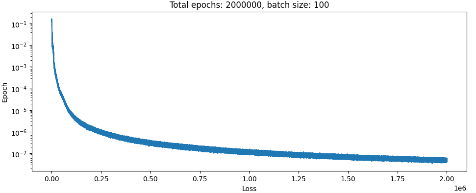Absolutely textbook. And here is what it looks like when the model does projection: I am stunned. The model was trained to predict the positions at t+1 from time t but here I made the model predict all 1000 sequential steps in succession, so the divergence here is the accumulated error. This is an astoundingly easy problem compared to what I was dealing with before.

Losses between timesteps:

Just for comparison here is what happens when you diff adjacent timesteps and plot the mean squared error for the first 1000 datasets: 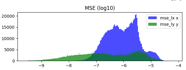So a model that has a mse of 1e-7 is doing ok, but could be better. We can see that there is quite a bit lower error in the y axis. This is a dataset of drops of water falling down so I assume that this is just the drop being close to stationary at the start.