This is just some quick measurements of the BH curves of the magnetic material used previously. I watched this typically excellent applied science video on how to do it. Here is an image of the setup, I added a new sense coil to see what’s going on:
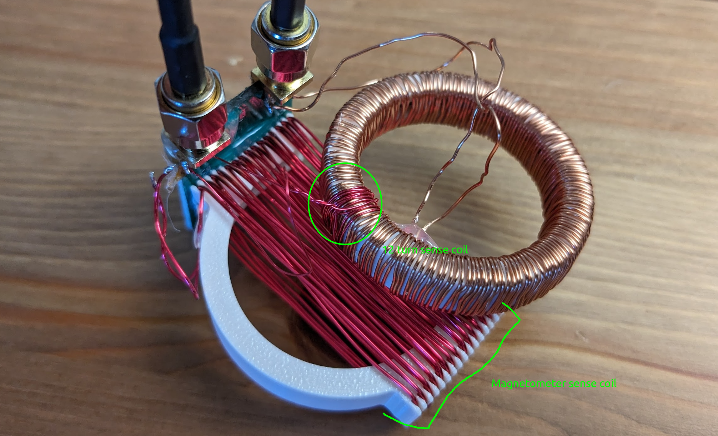
(For posterity: the coil has 12 loops in it.) The circuit to drive the coil looks like this:
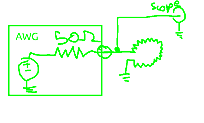
So I can figure out the current flowing through the coil using the known waveform of the AWG and the 50R impedance of the scope. The “triggering” of where the AWG waveform is is achieved by putting out a square wave on another channel of the AWG and then just using np.sin to generate what the inside of the AWG would have looked like. Beats a current probe or a current sens resistor, really.
Waveforms
Here is what a measurement looks like. I have normalised all the waves so they fit in the plot window nicely, the exact amplitudes aren’t important since they are all supposed to be different units anyway:
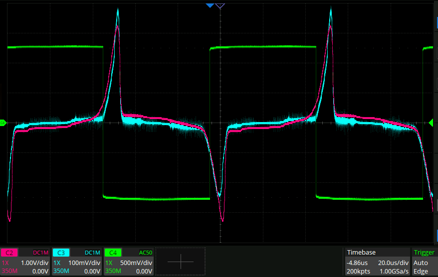
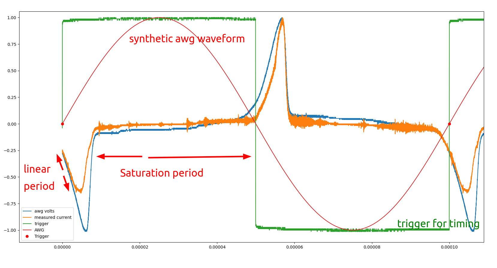 Or, on the scope:
10kHz
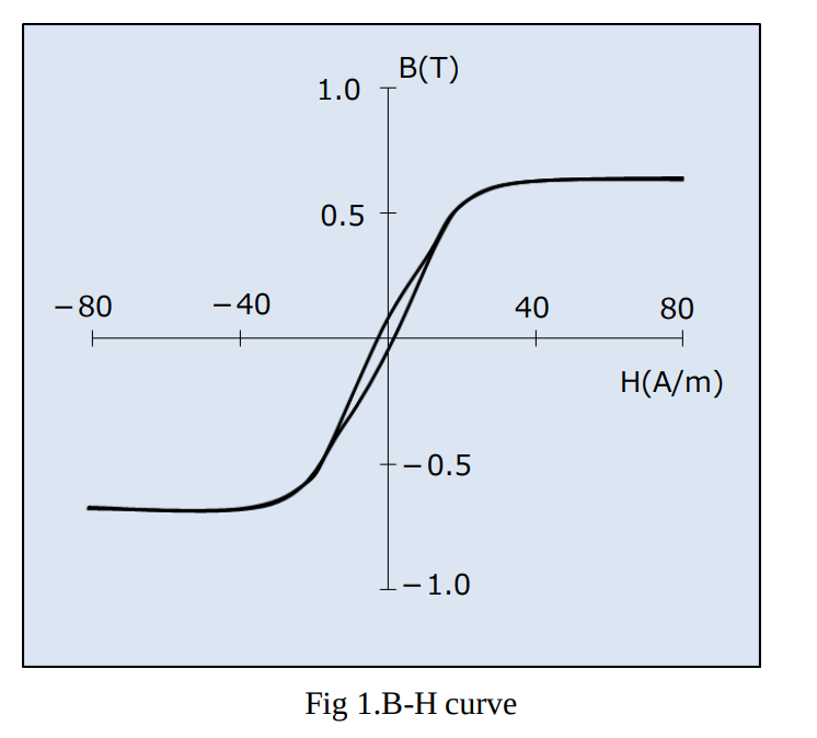
This is what the b-h curve looks like at 10kHz:
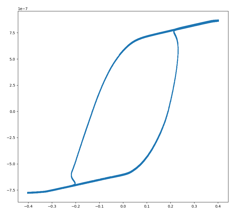
What utter absolute trash. Sheer garbage. what a Yuge hysteresis loop. I managed to find a product that is kind of designed for magnetometers, and its loop looks like this:
100kHz
This is the actual frequency of operation of the magnetometer:
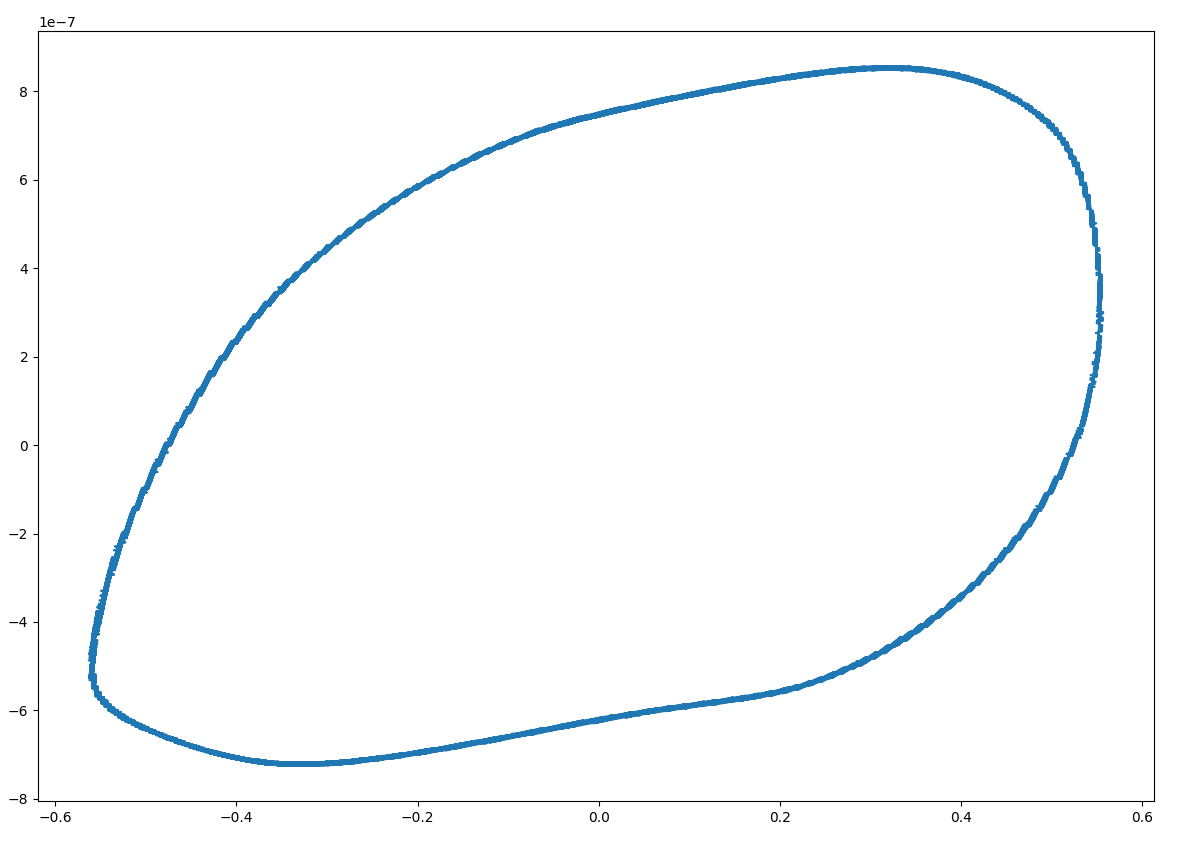
Absolutely comical. I must find something else.
Appendix: the script
import sys
import os
sys.path.append(os.path.join(os.path.dirname(__file__), '..', 'scope'))
import siglent_funcs as sf

import numpy as np
import matplotlib.pyplot as plt
from scipy import integrate

scope = sf.get_default_scope()

sample_rate, [awg_volts, current, trigger] = sf.get_samples_from_channels(scope, [2, 3, 4], 2e6)

edge_locs = np.argwhere((trigger[1:] > 0) & (trigger[:-1] <= 0)).flatten()

start = edge_locs[0]; stop = edge_locs[-1]
awg_volts, current, trigger = [x[start:stop] for x in [awg_volts, current, trigger]]
edge_locs = edge_locs - start
print(f"edge loc repeatability: {np.diff(edge_locs)}")

awg_out = np.zeros_like(awg_volts)
awg_amplitude = 20
awg_impedance = 50
for i in range(edge_locs.size - 1):
    len_ = edge_locs[i + 1] - edge_locs[i]
    awg_out[edge_locs[i]:edge_locs[i + 1]] = np.sin(np.linspace(0, 2 * np.pi, len_)) * awg_amplitude
awg_current = (awg_out - awg_volts) / awg_impedance
awg_current = -awg_current  # make the plot the right way around

magnetic_field = integrate.cumtrapz(current- np.mean(current), dx=1/sample_rate)
field_flatted = np.convolve(magnetic_field, magnetic_field[0:edge_locs[1]], mode='same')
magnetic_field = magnetic_field - np.polyfit(np.arange(len(magnetic_field)), field_flatted, 1)[0] * np.arange(len(magnetic_field)) - np.mean(magnetic_field)


plt.figure(figsize=(20, 10))
time_ = np.arange(awg_volts.size) * 1 / sample_rate
plt.plot(time_, awg_volts / np.max(awg_volts), label="awg volts")
plt.plot(time_, current / np.max(current), label="measured current")
plt.plot(time_, trigger / np.max(trigger), label="trigger")
plt.plot(time_, awg_out / np.max(awg_out), label="AWG")
plt.plot(edge_locs / sample_rate, np.zeros_like(edge_locs), 'ro', label="Trigger")
plt.legend()

plt.figure(figsize=(20, 10))
# plt.plot(time_, awg_current, label="AWG current")
plt.plot(time_[0:-1], magnetic_field, 'r--', label="magnetic field")

plt.figure(figsize=(20, 10))
plt.plot(awg_current[0:-1], magnetic_field)
plt.show()