20230608 Learning rate

I still haven’t gotten the N body simulation to do anything useful at all really so I am going back to simulating particulars. I have noticed that learning rate is very important (duh) and so far I have only used a constant one. Pytorch has lots of “learning rate schedulers” though that adjust it over time to various criteria.

Exponential decay

Let’s train a neural net to model this function:

    def fn(x):
        out = x[:, -1] * x[:, -2] / (1e-3 + x[:, -3]**2)

Here is is the structure of the net:

    class Net(torch.nn.Module):
        def __init__(self):
            super().__init__()
            hidden_size = 100
            self.input_conv = Linear(3, hidden_size)
            self.hidden_conv = Linear(hidden_size, hidden_size)
            self.output_conv = Linear(hidden_size, 1) 
            self.act = ReLU()
        def forward(self, x):
            x = self.act(self.input_conv(x))
            x = self.act(self.hidden_conv(x))
            x = self.output_conv(x)
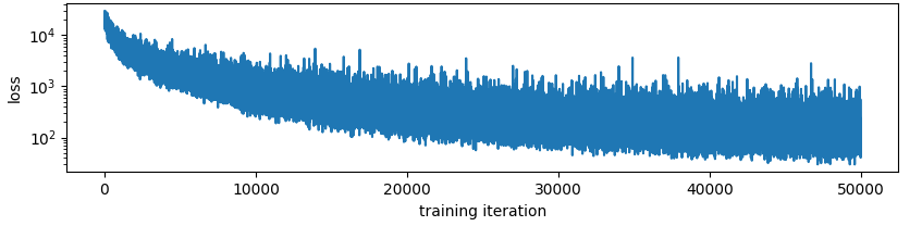
            return x

I trained it with a learning rate that decayed from 3e-1 to 3e-3 over 50k epochs, and the results look like this: 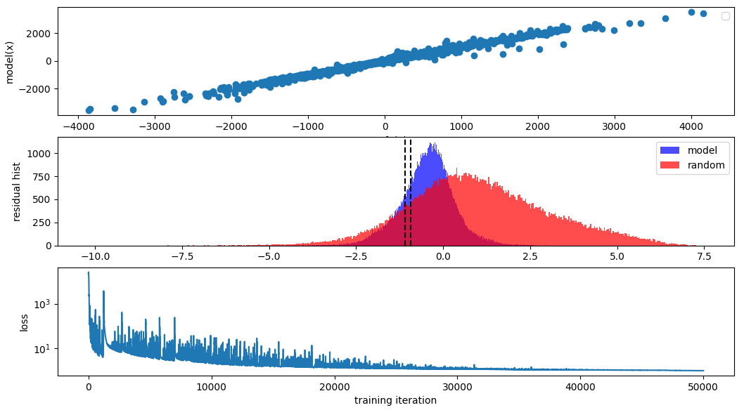So it did a somewhat reasonable job. But I noticed that the learning rate decay is both very important and not so trivial to get right. You can see at the beginning the variance in the loss is very high, indicating that perhaps too large of a step is being taken and at the end it is very low, indicating that perhaps the learning rate is too low. I wonder if there are any schedulers that attempt to maintain a constant variance (in log space) in the loss function. To me that sounds like a good way to get a signal about how big of a step size to take in the gradients. Wait no that makes no sense. As the model trained the loss function variance would not decrease. I guess maybe this works to find a good learning rate rather than to adjust it over time. The loss functions is most definitely not a random variable though, here is the loss over time zoomed in to the middle of the above training run: 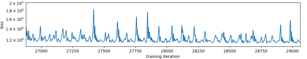Extremely periodic. I wonder if this has to do with the adam ‘momentum’.

Constant variance - good for picking?

So from the above loss function over time it looks like halfway between 3e-1 and 3e-3 is a good learning rate. Here is what happens to the loss function if you use 3e-2 for the whole training run: 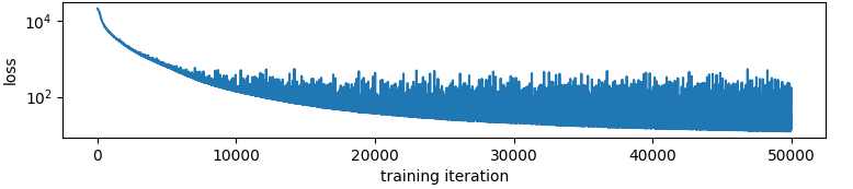The variance of the learning rate goes up! So maybe I am onto something here! Like I said though, the loss is not a random variable. This is what things looks like at the tail end: 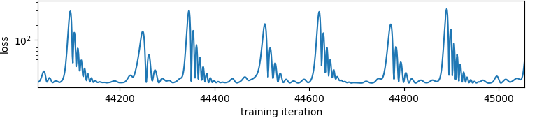not sure what the dealio with this is. I noticed that I was training on the same 10k examples over and over so I made it a different 10k each time. Here is the exact same training run, generating different samples for each forward pass: …Yeah there you go. Overfitting is happening somehow. I assumed this wouldn’t happen since the model has like 200 parameters in it and the input is a perfect random variable but I guess not. This still seems to exhibit the learning rate going up phenomenon though.

Experiment: Constant variance:

Here is the loss and the variance in the loss plotted as a function of epoch. The loss is calculated as the standardd deviation of the last 500 epochs. It looks like this: 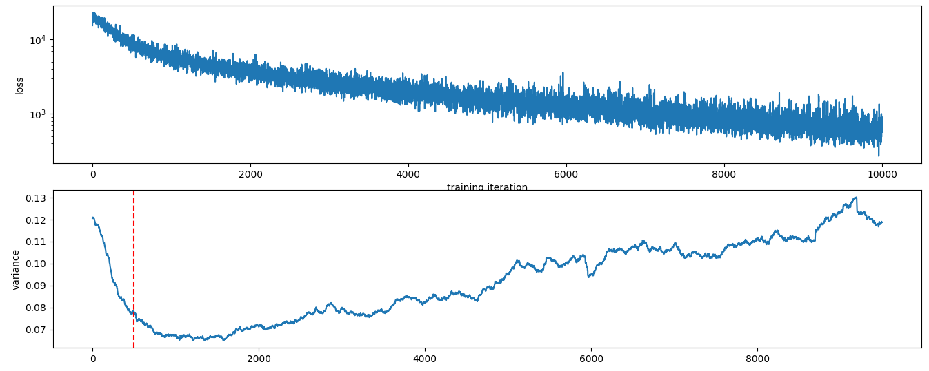This intuitively makes sense. The std is high at the beginning (because the std of a straight but sloped line is high) and then goes don until the first fast learning is done. Then it goes up gradually with time, as I observed before. The red vertical line is at 500, the width of the variance-estimating filter. Let’s try and control the variance to 0.075. 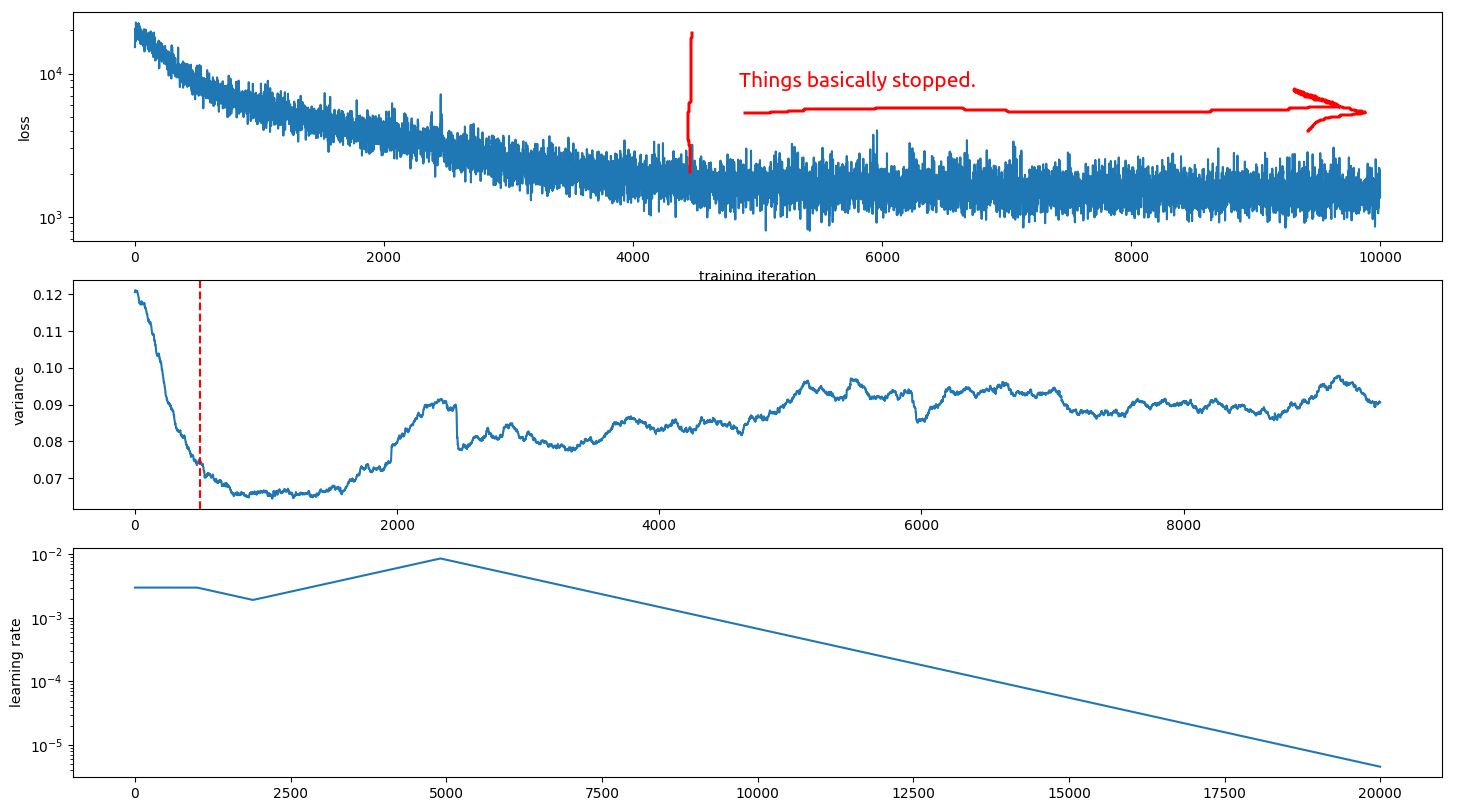Here’s how it went: Very poorly. It seems that the natural output of the model has a variance of at least 0.075 and so even if the learning rate is crushed to 0 then the variance still stays high. I didn’t expect that one… This perhaps explains why I don’t see anyone else doing this.

Variance within the model

There is a glimmer of hope for this idea still. If we know the variance within the model then we could perhaps subtract that out from the variance due to the too-high learning rate and then use that to adjust the learning rate. We have a batch size of 10k here, so we can get a quite accurate estimate of the models variance over time without too much extra computation.

Here is the variance in the model calculated as follows:

        x = torch.randn(40000, 3)
        y_model = model(x)
        y_gt = fn(x)
        loss = F.mse_loss(y_model, y_gt)
        loss.backward()
        model_stds.append(torch.std(torch.log10((y_model - y_gt)**2)).cpu().item())

Over time: 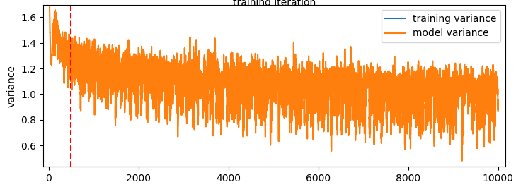So it doesn’t really change much over the course of the run. Note that it’s way higher than the variance of the losses here. This is because the variance of the losses above is calculated as std(log10(mean(errors))) whereas the model variance is std(log10(errors)). Regardless the main point here is that the models error spread in log space (% error spread) stays pretty constant over the training run.

Takeaway

• The measured variance of the loss curve over time is the combination of the natural variance in the models output and the additional variance due to updating the models weights according to the learning rate.
• As a model becomes better trained, the spread of its errors may in fact go up which is unintuitive to me.