Background
Recently I have been trying to train on this function:
    def fn(x, epsilon):
        out = x[:, -1] * x[:, -2] / (epsilon + x[:, -3]**2)
Using a very simple net structure like this one:
class Net(torch.nn.Module):
    def __init__(self):
        super().__init__()
        hidden_size = 100
        self.input_conv = Linear(3, hidden_size)
        self.hidden_conv = Linear(hidden_size, hidden_size)
        self.output_conv = Linear(hidden_size, 1)
        self.act = ReLU()

    def forward(self, x):
        x = self.act(self.input_conv(x))
        x = self.act(self.hidden_conv(x))
        x = self.output_conv(x)
        return x
With rather mixed results, to say the least. On thing that I noticed is that the choice of epsilon matters a huge amount here. This is very relevant to my gravitation simulations since of course gravitation involves the calculation of an inverse square of the distance between bodies. So if I can’t train a net to approximate this function, I can’t expect it to do well.
Experiments varying epsilon
Here are the results of training a net with different values of epsilon. Learning rate 3e-4, batch size 40e3:
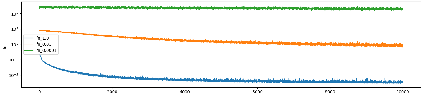 …So you can see here that if epsilon approaches any reasonable value stuff falls apart very quickly. Not only is the error high but the model stops actually being able to learn at all. This is what the error histograms look like:
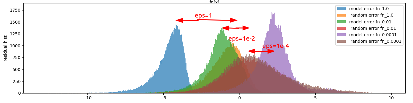 Interestingly when you get a small enough epsilon, the median error of the model is actually higher than the median error of two randomly selected inputs! This suggests to me that the fitness function is bad, but we shall experiment on that later.
Piecewise linear.
Since the activation function here is a Relu and there is only one hidden layer the model basically has to do a piecewise linear approximation. Let’s try training it on a deeper network and see if that makes a difference:
# Create network class
class Net(torch.nn.Module):
def __init__(self):
super().__init__()
hidden_size = 100
self.input_conv = Linear(3, hidden_size)
self.hidden_conv = Linear(hidden_size, hidden_size)
self.hidden_conv2 = Linear(hidden_size, hidden_size)
self.hidden_conv3 = Linear(hidden_size, hidden_size)
self.output_conv = Linear(hidden_size, 1)
self.act = ReLU()
def forward(self, x):
x = self.act(self.input_conv(x))
x = self.act(self.hidden_conv(x))
x = self.act(self.hidden_conv2(x))
x = self.act(self.hidden_conv3(x))
x = self.output_conv(x)
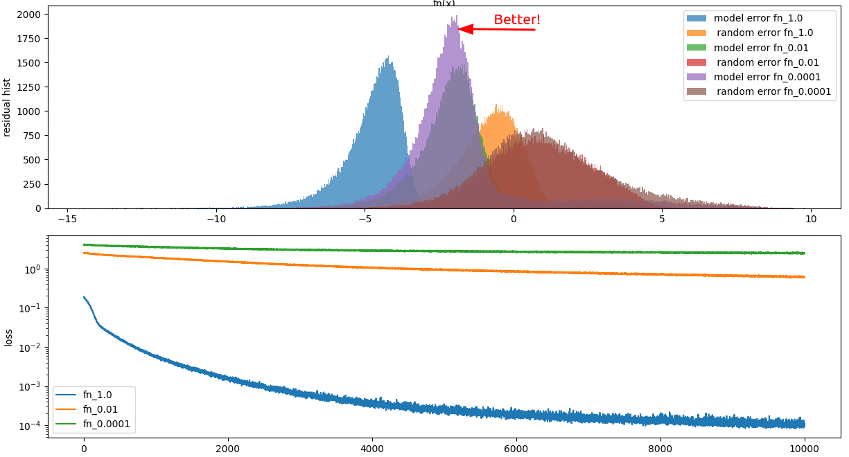
return xaaaand it’s not much different:
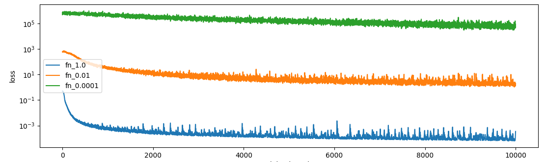 Although the loss of the 1e-4 epsilon actually does start going down, the median error of the model is still higher than two random points. I notice on the higher two epsilons the learning curves have signs of too high of a learning rate (those spiky bits) so I re-ran with 1e-4 learning rate, but that did not make that much of a difference.
Different loss function?
(In this section I went back to the one-hidden-layer model) The loss function that I have been using is mean squared error, cause I figured this was a fitting problem and those weirdo loggy loss functions are for cat detectors. Perhaps not though. I think what is happening here is the sharp point of the function where the denominator goes to 0 is dominating the loss curve. So if we optimised for the percentage error, or the ratio of the true / desired output then things would perhaps perform better. Here is a fitness function along those lines:
loss = F.mse_loss(torch.log(1 + torch.abs(y_model - y_gt)), torch.zeros_like(y_model))And here is how it performs:
 Success! The model actually trains and when we look at the histogram of the losses, we can see that the median model mean squared error is actually less than a random error!
The above loss function seems kind of hacky. I think that this one truly does represent the ratio of the input to output, whilst still preserving sign and whatnot:
Success! The model actually trains and when we look at the histogram of the losses, we can see that the median model mean squared error is actually less than a random error!
The above loss function seems kind of hacky. I think that this one truly does represent the ratio of the input to output, whilst still preserving sign and whatnot:
        def two_sided_log(x): return torch.sign(x) * torch.log(1 + torch.abs(x))
        loss = F.mse_loss(two_sided_log(y_model), two_sided_log(y_gt))
This is what we get training on just the 1e-4 model:
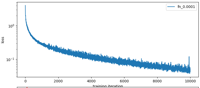 Amazing!
And a new visualisation: Let’s test the model on all ones, except for the denominator which ranges linearly from -1 to 1. We can think of this as a kind of partial derivative of the model with respect to the denominator I suppose:
Amazing!
And a new visualisation: Let’s test the model on all ones, except for the denominator which ranges linearly from -1 to 1. We can think of this as a kind of partial derivative of the model with respect to the denominator I suppose:
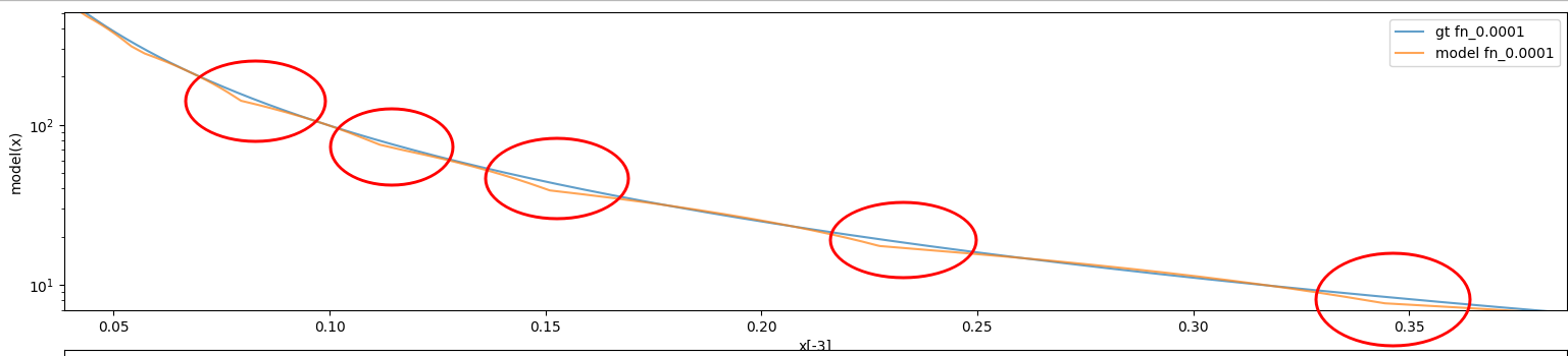
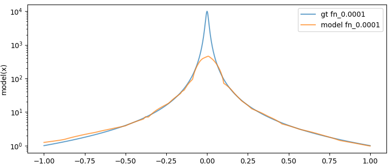 Looks reasonable. Note the log scale on the graph, the model is indeed fitting to percentage error. We can see the parts where the linear approximations are happening.
Here’s what the model looks like after 50e3 training runs. This is a closeup of the above graph. We can see here that the model is doing a bunch of linear approximations. I don’t think this is an artifact of the plotting that was used:
Looks reasonable. Note the log scale on the graph, the model is indeed fitting to percentage error. We can see the parts where the linear approximations are happening.
Here’s what the model looks like after 50e3 training runs. This is a closeup of the above graph. We can see here that the model is doing a bunch of linear approximations. I don’t think this is an artifact of the plotting that was used:
Sanity check
Here is the output of the regular mse loss trained model with the same visualisation:
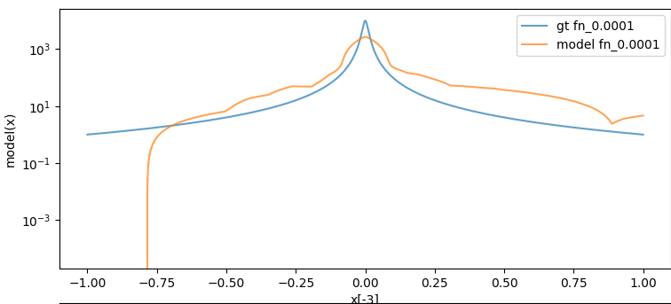 Hot garbage. I think my reasons are correct here. The error around x == 0 is actually a bit lower than the previously trained model (verified with mouseover in matplotlib). It’s just that this marginally lower absolute error here comes at the cost of hugely larger error everywhere else.
Sanity check: sane.
Hot garbage. I think my reasons are correct here. The error around x == 0 is actually a bit lower than the previously trained model (verified with mouseover in matplotlib). It’s just that this marginally lower absolute error here comes at the cost of hugely larger error everywhere else.
Sanity check: sane.
Going deeper
I had more troubles with the actual problem at hand, so I am back here. What about this fitness function:
loss = F.l1_loss((y_model - y_gt) / (1 + y_gt.abs()), torch.zeros_like(y_gt))It’s explicitly optimizing for the percentage error rather than via some mathematical curiosity. This is the error after 50k training runs:
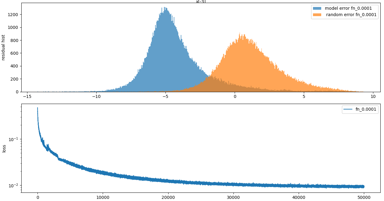 We can see the median log(MSE) is like -5 now, which is like 2.5OOM better than above.