20240618 Impedance network simulation

Background

The goal here was to build some kind of metal detector that could operate at a wide range of frequencies. Previous work here. It seems rather impractical/impossible(?) to make a coil that actually resonates across a decade+ frequency range of like 1-10kHz, ideally 100kHz. We want such a large frequency range because iron ore and so on has a quite different response vs frequency to gold, and so doing a full frequency sweep should provide a bunch of information.

Why resonate?

It’s obviously possible to put a whole bunch of energy in a tx coil across many frequencies via some kind of class-D amplifier setup. And you could open-circuit the rx coil and measure the voltage across it too, if you wanted. But I don’t think that that would be a good way to operate the device. Operating the coil with a capacitor in parallel as a tank circuit at the tx coil frequency is universally how metal detectors are designed, and with good reason I think. It is not so much that the tank circuit provides gain by resonating, but that it presents as a different impedance. It actually absorbs more of the energy in the oscillating magnetic field. So it’s not equivalent at all to sticking a super low noise amplifier on the output of the coil.

Briefly: Why not operate at different frequencies sequentially?

<<<<<<< HEAD You could trivially design a setup that used a switched capacitor network or tapped off the inductor to operate at different frequencies sequentially. I find this to be against the ideals of the project and refuse on that basis. When I think about what a good metal detector should be doing it is blasting the environment with as much wideband energy as it possibly can on the tx side, and using some kind of multiple coil setup to get even more information a la phased array. So since wideband seems not to be possible, perhaps N-band is.

Setup:

So one way to get this to work would be to just have a whole pile of different receive coils all operating at once. That seams infeasible though. If you look at the actual physical size of metal detector coils, they are pretty big. Big enough that stacking 10 of them together probably wouldn’t be a super great idea. What if instead of this we could have one very large coil and then operate different subsections of it at different frequencies?

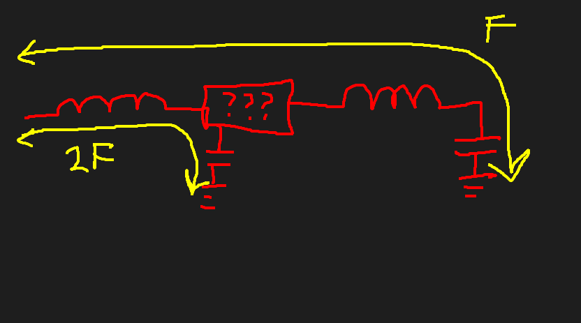
It would work something like this: Suppose you have a coil, and divide it into two sections, connected in series. The two sections together would resonate at some frequency F, and the subsection at the end would resonate at some frequency 2F. Obviously if you just hooked this up as-is, it wouldn’t work. But, what if you inserted a magic device in the middle? A device that let frequency F through, but blocked frequency 2F. Then the smaller section of the coil would be ‘invisible’ to the larger section, and they could resonate at both frequencies at once! #diagram here#

What would this look like?

Well it would look a little bit like a diplexer in the sense that different frequencies go to different places. It would actually need three ports I think, with the third port being used to attach the capacitor for the 2F resonator.

I don’t really know how to design such a thing, but how hard could it be to simulate?

Simulation of a graph of RLC networks.

So we have N inductors, resistors, and capacitors connected together in a graph. And we want to calculate the impedance between the nodes as a function of frequency. The term for this is ‘Nodal analysis’, and it involves at some point constructing an ‘Admittance matrix’.

The physical layout of the system can then be described then as an adjacency matrix where the N nodes in our system are connected by resistors and capacitors. Note that for reasons I don’t have a great intuition for, ground does not count as a node when doing these kinds of analyses. Instead, a connection from a node i to ground is represented as a connection with itself i.e. an element on the matrix diagonal.

if $v=ir$ and we define admittance of something to be the inverse of the resistance to be $y=1/r$. Then $yv=i$, obviously. It transpires then that we can write our Admittance Matrix $Y$ like this: $YV=I$ Where when we have N nodes Y is the NxN admittance matrix, $V$ is the Nx1 voltages of the different nodes, and $I$ is the Nx1 currents in the nodes. If we knew the currents going into and out of the nodes then, we could solve for the voltages like this: $V=Y^{-1}I$ OK. This is all lecture note stuff. But recall that we don’t have ground as an explicit node here. That means that we can stuff 1A of current into node 0 without having to have a -1A anywhere else as the current will just end up going to ground. So if we say that the input node is node 0 and we have N nodes, then $I=[1,0,\mathrm{0...}{0}_n].T$. We know the admittance matrix, we know about torch.pinv, and we know what I is! The system is now solveable

======= You could trivially design a setup that used a switched capacitor network or tapped off the inductor to operate at different frequencies sequentially. You could then build up a picture of what is happening by scanning through the frequencies one after the other, but this would of course take a lot longer. I find this to be against the ideals of the project and refuse on that basis. When I think about what a good metal detector should be doing it is blasting the environment with as much wideband energy as it possibly can on the tx side, and using some kind of multiple coil setup to get even more information a la phased array. But since wideband seems not to be possible, perhaps N-band is.

f591c9a2091b738c4a6b96dc61d5e7a703aa10a3

Simultaneous multi-frequency inductors:

So one way to get this to work would be to just have a whole pile of different receive coils all operating at once. That seams infeasible though. If you look at the actual physical size of metal detector coils, they are pretty big. Big enough that stacking 10 of them together probably wouldn’t be a super great idea. What if instead of this we could have one very large coil and then operate different subsections of it at different frequencies?

It would work something like this: Suppose you have a coil, and divide it into two sections, connected in series. The two sections together would resonate at some frequency F, and the subsection at the end would resonate at some frequency 2F. Obviously if you just hooked this up as-is, it wouldn’t work. But, what if you inserted a magic device in the middle? A device that let frequency F through, but blocked frequency 2F. Then the smaller section of the coil would be ‘invisible’ to the larger section, and they could resonate at both frequencies at once!

What would this look like?

Well it would look a little bit like a diplexer in the sense that different frequencies go to different places. It would actually need three ports I think, with the third port being used to attach the capacitor for the 2F resonator.

I don’t really know how to design such a thing, but how hard could it be to simulate?

Simulation of a graph of RLC networks.

So we have N inductors, resistors, and capacitors connected together in a graph. And we want to calculate the impedance between the nodes as a function of frequency. The term for this is ‘Nodal analysis’, and it involves at some point constructing an ‘Admittance matrix’.

The physical layout of the system can then be described then as an adjacency matrix where the N nodes in our system are connected by resistors and capacitors. Note that for reasons I don’t have a great intuition for, ground does not count as a node when doing these kinds of analyses. Instead, a connection from a node i to ground is represented as a connection with itself i.e. an element on the matrix diagonal.

If $v=ir$ and we define admittance of something to be the inverse of the resistance to be $y=1/r$. Then $yv=i$, obviously. It transpires then that we can write our Admittance Matrix $Y$ like this: $YV=I$ Where when we have N nodes Y is the NxN admittance matrix, $V$ is the Nx1 voltages of the different nodes, and $I$ is the Nx1 currents in the nodes. If we knew the currents going into and out of the nodes then, we could solve for the voltages like this: $V=Y^{-1}I$ OK. This is all lecture note stuff. But recall that we don’t have ground as an explicit node here. That means that we can stuff 1A of current into node 0 without having to have a -1A anywhere else as the current will just end up going to ground. So if we say that the input node is node 0 and we have N nodes, then $I=[1,0,\mathrm{0...}{0}_n].T$. We know the admittance matrix, we know about torch.pinv, and we know what $I$ is! The system is now solveable! Yay!

Code

Network representation

Obviously we want to represent the graph of the network by storing the component values (like 100e-9 is a 100nF inductor). So this means that the adjacency matrix is actually a 3xNxN matrix, with the first dimension being [R, L, C]. Then for a given frequency we can calculate the impedances of the different components and put them in parallel (not sum!) across the first dimension. It looks like this:

def calc_impedance(freq, grid):
    """Calculate the impedance matrix from the component grid.
 
    B * 3 * N * N adjacency matrix for (inductance, capactitance) for a network of N nodes.
    It is assumed that only one of the adjacency matrix edges is populated.
    Connections from a node to iself is how connections to ground are represented.
    Returns a B*N*N impedance matrix for the network.
    """
    assert(freq.ndim == 2)
    assert(grid.shape[-1] == grid.shape[-2])
 
    B, _, N, _ = grid.shape
    j_omega = (1j * 2 * np.pi * freq).unsqueeze(1)
    # swap B idx for easier indexing into RLC:
    Z_lc = torch.zeros((RLC, B, N, N), dtype=torch.cfloat)
    nonzero = torch.permute(grid != 0, (1, 0, 2, 3))
    Z_lc[R, nonzero[R]] = grid[:,R][nonzero[R]].cfloat()
    Z_lc[L, nonzero[L]] = (j_omega * grid[:,L])[nonzero[L]]  # Reactance for inductors
    Z_lc[C, nonzero[C]] = 1 / ((j_omega * grid[:,C])[nonzero[C]])  # Reactance for capacitors
 
    # sum the RLC's in parallel:
    admittance = torch.zeros_like(Z_lc, dtype=torch.cfloat)
    admittance[Z_lc != 0] = 1 / Z_lc[Z_lc != 0]
    admittance = admittance.sum(axis=0)
    # Add the transpose to itself apart from the diagonal elements to make the matrix symmetric.
    # if an impedance connects node i to node j, it should also connect node j to node i.
    admittance_sym = admittance + torch.transpose(admittance * (1 - torch.eye(N)), -1, -2)
 
    Z = torch.zeros((B, N, N), dtype=torch.cfloat)
    Z[admittance_sym != 0] = 1 / admittance_sym[admittance_sym != 0]
    return Z

So this gives you your Z matrix from which the Y matrix can be constructed. That looks like this:

 
def calc_voltages(Z, I, get_residual=False):
    """
    Z is B*N*N impedance matrix for the network with N nodes (not including ground).
    I is B*N length current vector for the network.
    return V, a N length voltage vector for the network.
    """
    # broadcasting for convenience:
    if Z.ndim == 2:
        Z = Z.unsqueeze(0)
        return calc_voltages(Z, I, get_residual).squeeze(0)
    if I.ndim == 1:
        I = I.unsqueeze(0)
        return calc_voltages(Z, I, get_residual).squeeze(0)
    assert Z.ndim == 3 and I.ndim == 2
 
    Y = torch.zeros_like(Z, dtype=torch.cfloat)
    Y[Z != 0] = 1 / Z[Z != 0]
    # linear components, so the matrix should be symmetric
    # assert ((Y - torch.transpose(Y, -2, -1)).abs().sum() < 1e-6).all()
 
    # Sum admittances for each node
    # Y_diag = torch.diag(torch.sum(Y, dim=-1))
    Y_diag = torch.diag_embed(torch.sum(Y, dim=-1), dim1=-2, dim2=-1)
 
    # Constructing the network admittance matrix correctly
    eye_inv = (1 - torch.eye(Y.shape[-1])).unsqueeze(0)
    Y_network = Y_diag - Y * eye_inv
 
    # Solve for voltages using the network admittance matrix
    Y_inv = torch.linalg.pinv(Y_network)
    # Y_inv = torch.tensor(np.linalg.inv(Y_network.cpu().numpy()))
    V = Y_inv @ I.unsqueeze(-1).cfloat()
    residual = ((Y_inv @ Y_network).abs().max(dim=0).values - torch.eye(Y_network.shape[-1])).abs().sum()
    if residual > 0.1:
        print(f"Warning, bad residual! {residual}")
    # assert residual < 0.1
    # print("Residual:", residual.item())
    if get_residual: return V, residual
    return V

Example filter:

Bandpass filter:

here is an example bandpass filter from the extremely excellent LC filter design tool. I chose it as it was nice and complicated :)

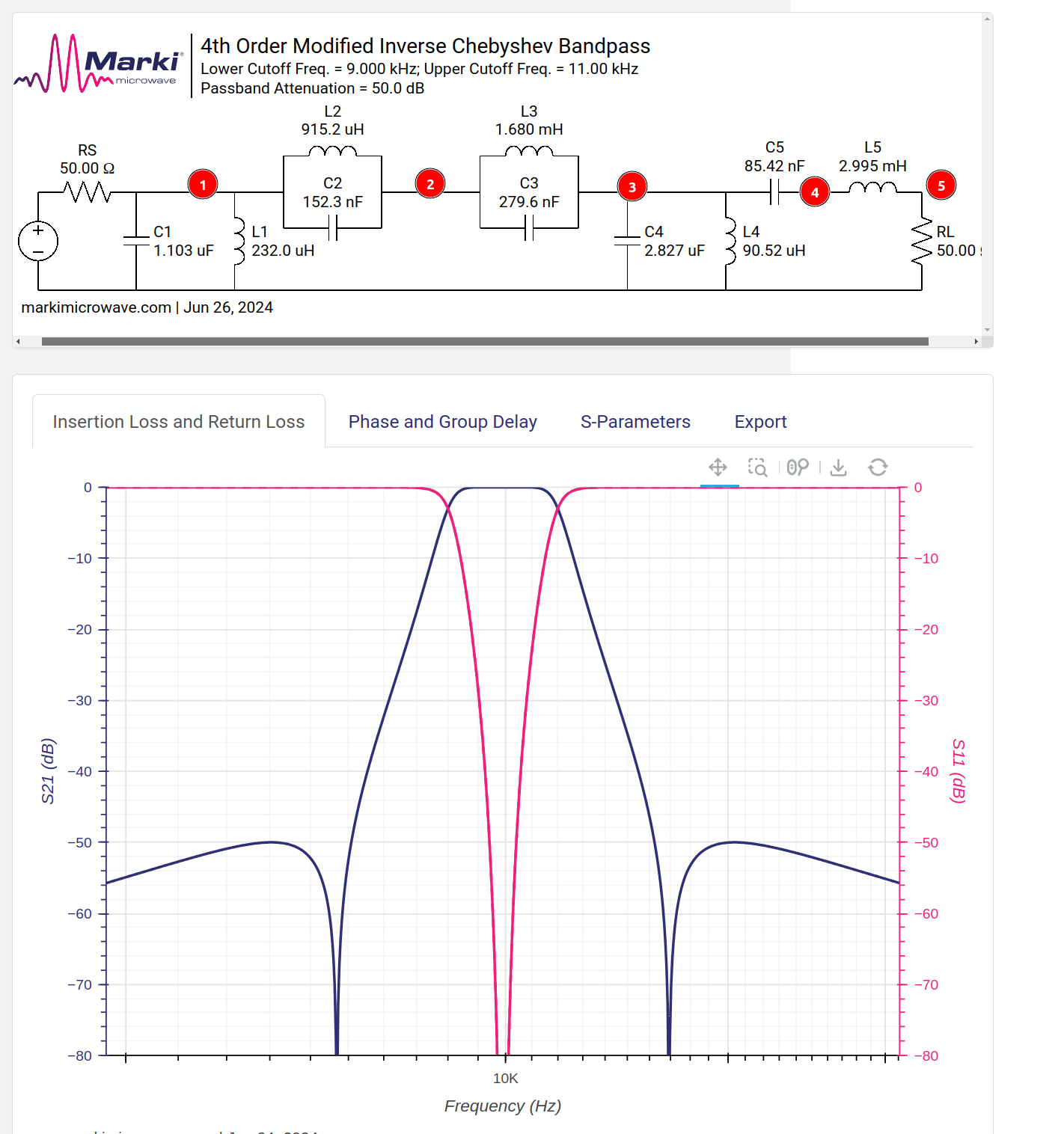
This is what the internal representation looks like. Translated with ChatGPT (which got all the connections wrong):

def setup_inverse_chebyshev_bandpass():
    grid = torch.zeros(3, 5, 5, dtype=torch.float)
    grid[R, 0, 0] = 50
    grid[C, 0, 0] = 1.103e-6   # C1
    grid[L, 0, 0] = 232.0e-6   # L1
    grid[C, 0, 1] = 152.3e-9   # C2
    grid[L, 0, 1] = 915.2e-6   # L2
    grid[C, 1, 2] = 279.6e-9   # C3
    grid[L, 1, 2] = 1.680e-3   # L3
    grid[C, 2, 2] = 2.827e-6   # C4
    grid[L, 2, 2] = 90.52e-6   # L4
    grid[C, 2, 3] = 85.42e-9   # C5
    grid[L, 3, 4] = 2.995e-3   # L5
    grid[R, 4, 4] = 50
    I = torch.tensor([1.0, 0.0, 0.0, 0.0, 0.0])
    return grid, I

And then the results look like this:

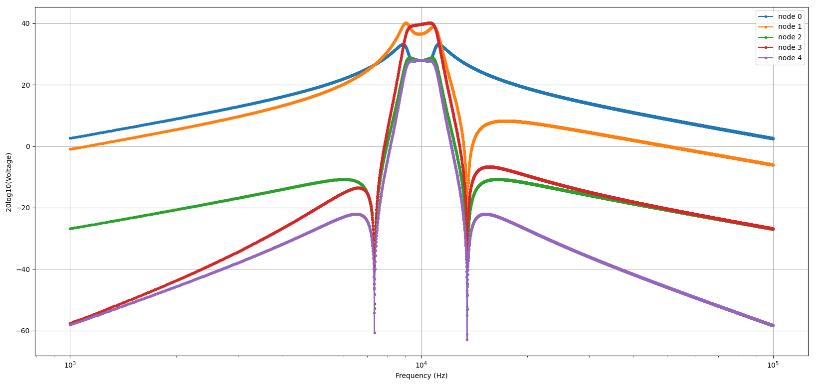
It looks very similar! The node of interest here is Node 4, the output node. But the scale seems off, this has a peak of 40dBV somehow. That’s because the circuit is 50Ohm terminated and we pushed 1A into it.

Optimisation

Now that we have a simulation that does a fantastic job of simulating these RLC networks, we can get to work optimising one for the job at hand. Since all the code is written in pytorch, we should be able to just gradient descent our way to the correct solution, right?

Method 1: gradient descent

def optimise_grad_lowpass():
    grid_gt, I_gt = setup_lowpass()
    # frequencies = torch.logspace(torch.log10(torch.tensor(1000)), torch.log10(torch.tensor(1e6)), 1000)
    frequencies = torch.linspace(8e3, 12e3, 100)
    V_gt = simulate_across_freq(grid_gt, frequencies, I_gt)
    
    grid, I = setup_lowpass()
    I = I.unsqueeze(0)
    # grid[grid != 0] = torch.randn_like(grid[grid != 0])
    grid[grid != 0] *= torch.rand(grid[grid != 0].shape) * 1e-2 + 1.0
    grid.requires_grad = True
 
    optimizer = torch.optim.SGD([grid], lr=1e-12)
    losses = []
    while True:
        optimizer.zero_grad()
        V , residual = simulate_across_freq(grid, frequencies, I, get_residual=True)
        # loss = torch.mean((V - V_gt).abs())
        # loss = torch.abs(torch.mean(1 - V.abs() / V_gt.abs())) + torch.abs(torch.mean(1 - V_gt.abs() / V.abs())) + residual * 10
        loss = torch.mean((V.abs() - V_gt.abs()) ** 2) / V_gt.abs().mean() + 100 * residual
 
        loss.backward()
        optimizer.step()
        losses.append(loss.item())
        print(f"iter {i}, loss: {loss.item():.3f}, means:{V.abs().mean():.3f}, {V_gt.abs().mean():.3f}, residual: {residual:.3f}")

This code absolutely refuses to converge or do anything useful. The loss blows up in two iterations with a 1e-12 learning rate. Notice that I initialized the matrix to something useful. One thing I noticed was that the optimisation process here had a tendency to produce matrices that did not invert very well. That is, $A{A}^{-1}!=I$. I had the brilliant idea of adding this residual to the loss function so that it would produce an invertable matrix alongside one that satisfied the other properties but that didn’t help.

Method 2: Genetic algorithm

 
def optimise_genetic_lowpass():
    grid_gt, I_gt = setup_highpass()
    Gsz = grid_gt.shape[-1]
    nf = 10
    frequencies = torch.linspace(7e3, 15e3, nf)
    V_gt = simulate_across_freq(grid_gt, frequencies, I_gt).squeeze().abs()
    
    grid, I = grid_gt.clone(), I_gt.clone()
    gsz = grid.shape[-1]
 
    popsz = 100
    grid_pop = torch.tile(grid.unsqueeze(0), [popsz, 1] + [1] * grid.ndim)
    grid_pop[grid_pop != 0] = torch.rand(grid_pop[grid_pop != 0].shape) + 0.1
 
 
    I_pop = torch.tile(I.unsqueeze(0), [popsz, nf] + [1] * I.ndim)
    frequencies_pop = torch.tile(frequencies.unsqueeze(0), [popsz, 1])
    frequencies_flat = einops.rearrange(frequencies_pop, 'n f -> (n f) 1')
    I_flat = einops.rearrange(I_pop, 'n f g -> (n f) g')
 
    def vis(frequencies, V_gt, V_meas, grid_pop, grid_gt):
        plt.figure(figsize=(7, 21))
        plt.subplot(311)
        plt.plot(frequencies, V_gt)
 
    old_grids = []
    errors = []
    best_errors = []
    while True:
        grid_expanded = torch.tile(grid_pop, [1, nf, 1, 1, 1])
        grid_flat = einops.rearrange(grid_expanded, 'n f a b1 b2 -> (n f) a b1 b2', n=popsz, f=nf, a=RLC, b1=gsz, b2=gsz)
        Z = calc_impedance(frequencies_flat, grid_flat)
        V_meas = calc_voltages(Z, I_flat).abs()
        V_pop = einops.rearrange(V_meas, '(n f) g 1 -> n f g', n=popsz, f=nf, g=gsz)
        r1 = (V_pop / V_gt.unsqueeze(0)).mean(dim=(-1, -2)) # Should be average across freq, dot against nodes we care about
        r2 = (V_gt.unsqueeze(0) / V_pop).mean(dim=(-1, -2))
        error = (r1 + r2) / 2
 
        order = torch.argsort(error, dim=0)
        error_sorted = error[order]
        grid_pop = grid_pop[order]
 
        best_error = error_sorted[0]
        es = [f"{x:.3f}" for x in error_sorted[0:10]]
        print(f"best error min: {error_sorted.min()}, e:{es}")
        frac = 2
        nkeep = popsz // frac; assert popsz % frac == 0
        grid_pop = torch.tile(grid_pop[:nkeep], [frac, 1, 1, 1, 1])
 
        error_scale = min(1, best_error)
        valid = grid_pop[nkeep:] != 0
        # mutation = torch.abs(torch.randn_like(grid_pop[nkeep:][valid]) * error_scale)
        mutation = (torch.rand(size=grid_pop[nkeep:][valid].shape)* 1.5 + 0.5) * error_scale
        mask = torch.randint(0, 10, mutation.shape) < 4
        mutation[~mask] = 1
        grid_pop[nkeep:][valid] *= mutation
 
        if len(errors) > 10 and np.std(np.array(errors)[-10:]) < 1e-5:
            if best_error < 1.1:
                print("ding")
            print("converged, refreshing")
            old_grids.append(grid_pop.clone())
            grid_pop[grid_pop != 0] = 10 ** (-12 * torch.rand(grid_pop[grid_pop != 0].shape) )
            errors = []
            best_errors.append(best_error)
        errors.append(best_error)
 

This had much more success. It converged in a few seconds for an RC filter to the correct values. But, for a more complicated net like a highpass filter it kept converging to values that weren’t very good. It seems as though it keeps getting stuck in a local minimum. So at the bottom of the loop there when I detect that the optimisation process has stopped I restart with fresh random values. It only takes a few seconds to converge so many starting points can be tested.

Overnight run

I did an overnight run of the highpass filter:

def setup_highpass():
    grid = torch.zeros(RLC, 3, 3, dtype=torch.float)
    grid[R, 0, 0] = 50
    grid[L, 0, 0] = 693.9e-6  # L1
    grid[C, 0, 1] = 232.1e-9  # C2
    grid[L, 1, 1] = 402.9e-6  # L3
    grid[C, 1, 2] = 232.1e-9  # C4
    grid[L, 2, 2] = 693.9e-6  # L5
    grid[R, 2, 2] = 50
    I = torch.tensor([1.0, 0.0, 0.0])
    return grid, I

Which gave me this histogram of errors. Each datapoint is one run of the optimisation process, so you can see that there are a couple of discrete different losses that get converged on.

It looks like there are a few runs here that converged to the right answer! The minimum error here was 1.0002.

Comparison Table

Here is a table of the actual grid of impedances for the ground truth and what the net managed to converge to. They are pretty much the same:

Best Convergence			Ground Truth
Resistance
4.95e+01	0.00e+00	0.00e+00	5.00e+01	0.00e+00	0.00e+00
0.00e+00	0.00e+00	0.00e+00	0.00e+00	0.00e+00	0.00e+00
0.00e+00	0.00e+00	5.01e+01	0.00e+00	0.00e+00	5.00e+01
Inductance
7.23e-04	0.00e+00	0.00e+00	6.94e-04	0.00e+00	0.00e+00
0.00e+00	4.11e-04	0.00e+00	0.00e+00	4.03e-04	0.00e+00
0.00e+00	0.00e+00	7.20e-04	0.00e+00	0.00e+00	6.94e-04
Capacitance
0.00e+00	2.20e-07	0.00e+00	0.00e+00	2.32e-07	0.00e+00
0.00e+00	0.00e+00	2.31e-07	0.00e+00	0.00e+00	2.32e-07
0.00e+00	0.00e+00	0.00e+00	0.00e+00	0.00e+00	0.00e+00

8 hour work run of more complicated filter

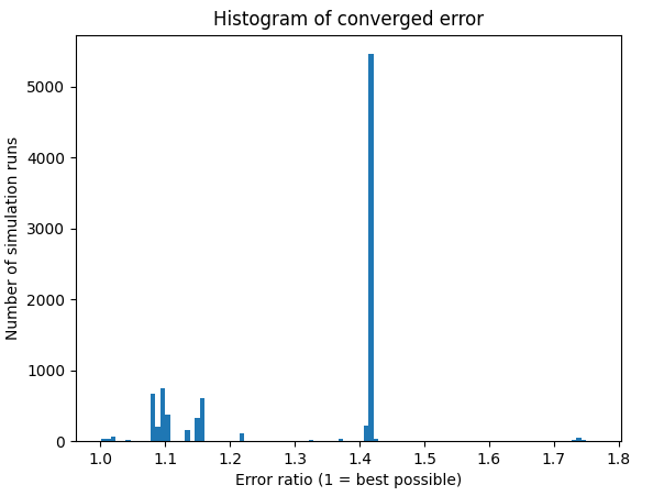
Here I tried a run over a ~10 hour workday, a much more complicated filter from above. That gave me this histogram of converged errors:

Histogram of converged errors:

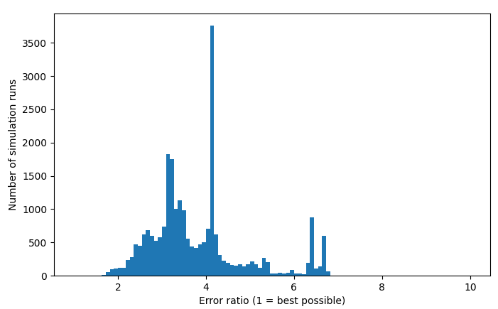
This one seems like a much more continuous distribution, not quite so many discrete modes. It also never converges to the right answer, with a pretty high minimum error.

This isn’t looking so crash hot. I suppose it makes sense that this kind of landscape of L’s an C’s would be a minefield of local minima and that it would be difficult to converge on the global minima. I don’t necessarily need the global minima for my application but the miserable failure here hardly bodes well…