A good introduction and guide on how to make a fluxgate magnetometer can be found in the Wireless world magazine, 1991. I didn’t really follow the guide but if you read it you’ll get the general idea.

Version 1

The idea of winding a toroid sounded too hard to me so I made two separate linear coils and connected them with some magic magnetic tape. Here are the two windings before I added the sense coil:

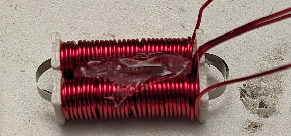
And here is what it looks like “fully assembled”:

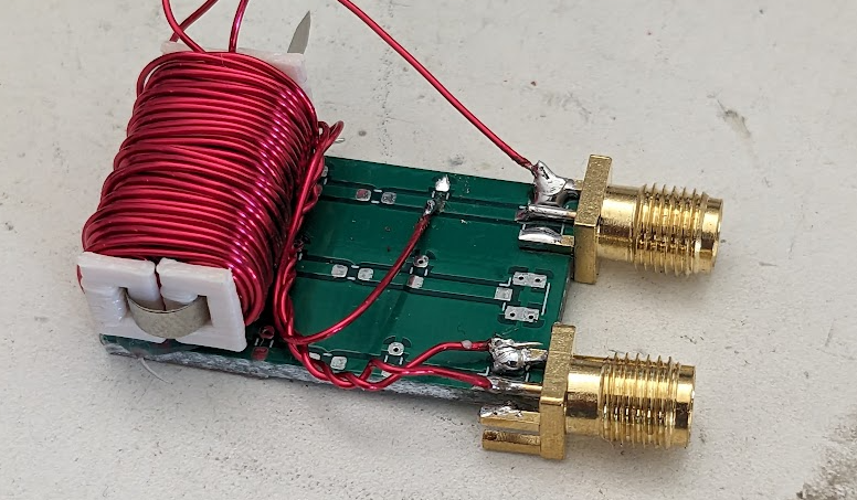
I drove it straight out of the signal generator and amazingly it worked out of the box. It’s quite sensitive and was able to detect my twiddling of a bar magnet like 5 meters away! This is quite significant as it represents the first time I have ever built an electronic device and had it (1) work on the first try and (2) had it be more sensitive than expected. I suppose it makes sense now how they were able to get them good enough in WWII to detect submarines from a plane.

The limit on the detection though was the 0 level. Even when I aligned the sensor such that it was normal to the ambient magnetic field, there was still quite a large signal measured on the scope. Reading around a bit (“Magnetic sensors and magnetometers” is a sensible book) it seems that one of the main reasons to use a toroid is that it evens out the variations in manufacturing that are the result of these residual errors.

Since the magnetometers measurement comes from the asymmetry in how each side of the device magnetises/demagnetises, it makes sense that this would be worth switching the design.

Version 2

So, time to suck it up and wind a toroid. The book also mentioned that one way to get low variation in your wound toroid is to wind it such that there windings are just touching along the inner race, since then the wire diameter is what sets the pitch. Good advice but that results in far more windings than is required in practice and I realised just after I started winding that I could have printed some notches in my 3D print which would have also defined the winding spacing and not required me to wind 7m of wire through a 35mmID toroid. Oh well.

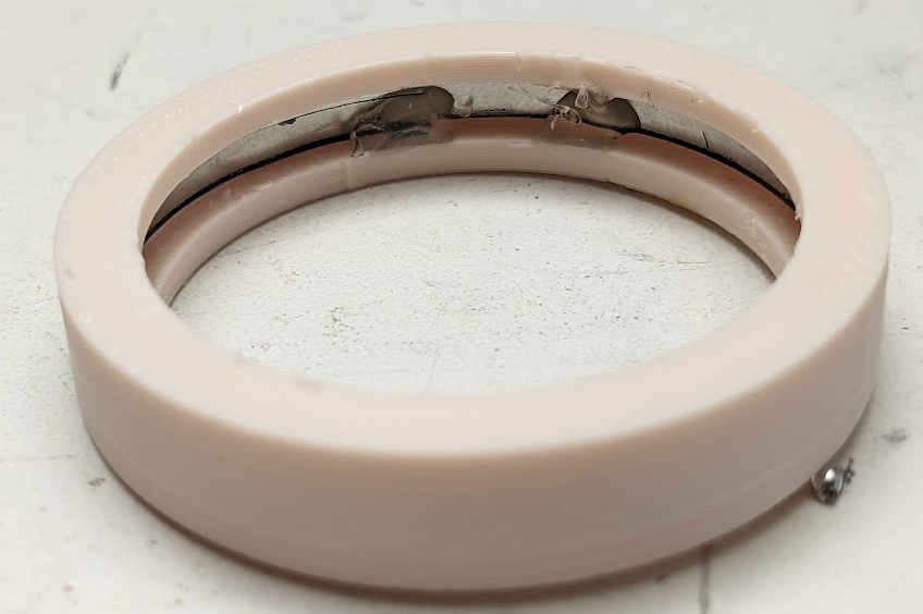
Toroid construction

Here is the inside of the toroid. I put two strips of metal ~2.75mm wide (hand cut with scissors, naturally) into the toroid which was sized to just fit the length of the strip.

And here it is all wound together:

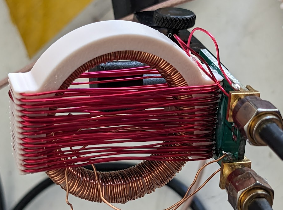
…Not exactly a precision device, is it? But the 3d printed outer sense coil winding is critical. By rotating the inner toroid with respect to the outer one, I can move it to a point that minimizes the measurement when the sensor is perpendicular to the earths field. This makes quite a bit of difference.

Zero field

Here is the output of the sensor, showing the maximum, minimum, and zero measurements achievable here on earth:

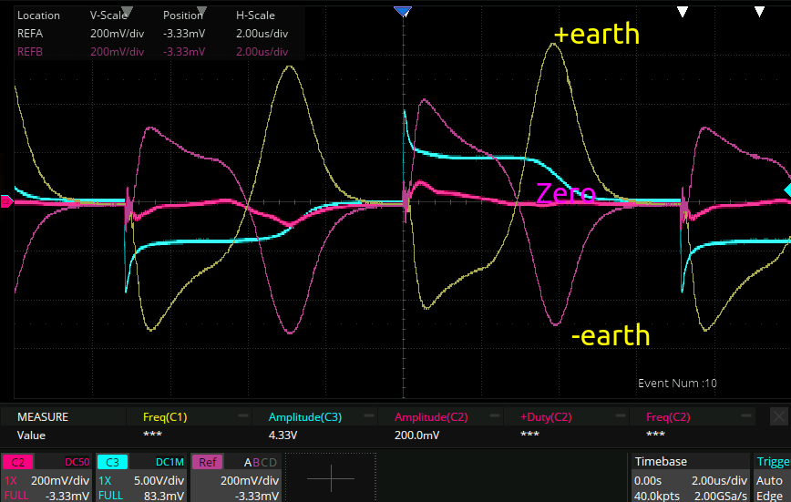
So that’s (3.2 - -2.5) / 55e-6 = 100mV/uT. That’s 103kV/tesla, which sounds good. That’s also 10000 gamma/volt, and the above magazine article calibrates it to a maximum of 100 gamma/volt, or 100x more sensitive.

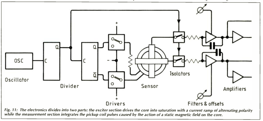
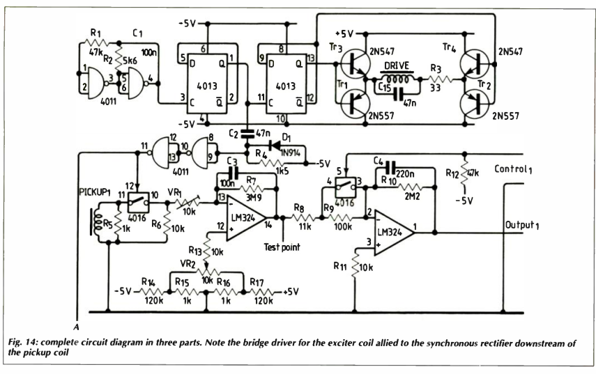
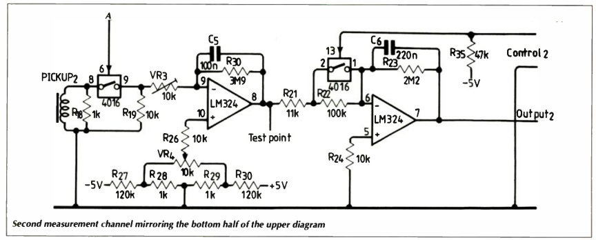
Magazine schematic:

Gating and filtering

Here’s an idea: The signal has 0 DC level. So what we really want to do here is rectify it. But, the signal is small. So instead we can just grab the section of the signal that has the spike in it, and average around that!

Like this:

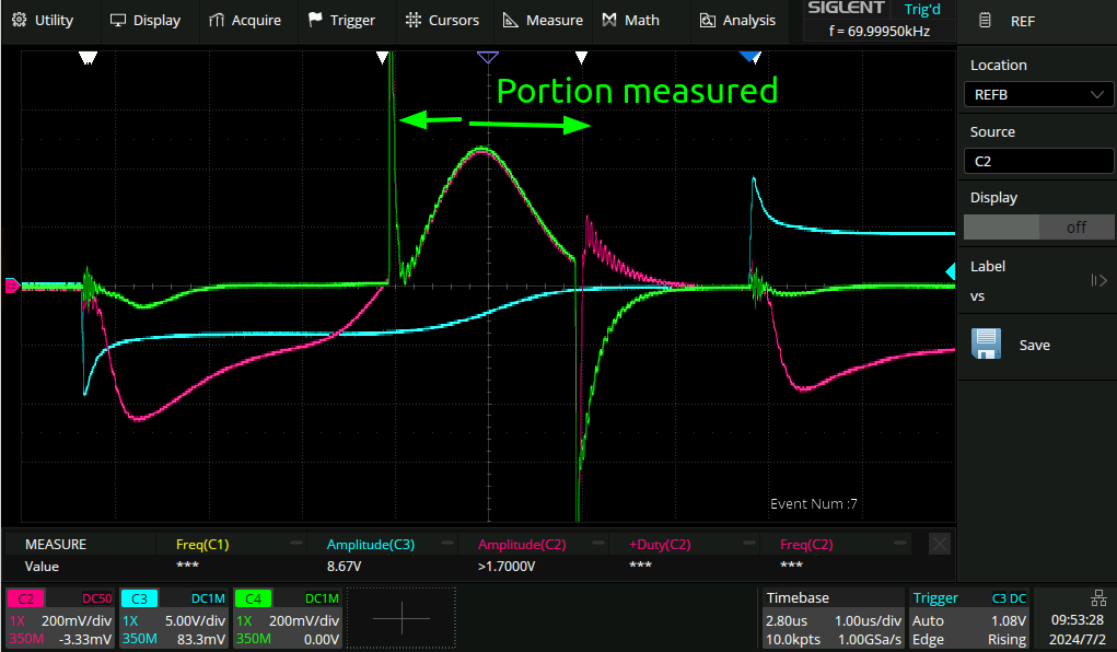
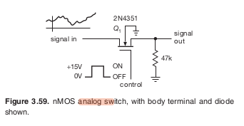
ta-da! Done using an SI2302 analog switch, aka a mosfet as recommended by the Art of Electronics:

It introduces a huge amount of charge injection but I’m going to wave my hands and say it’s fine since the + and - section average to 0 anyway. Filtering this chopped signal and zooming into the noise floor, we get:

Which sure does look an awful lot like mains. So I guess we have reached the noise floor of this particular environment.

Alternative to gating and filtering

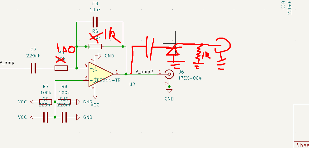
I got annoyed at the above gating because of the charge injection that I couldn’t get rid of. I tried adding a complementary pmos and when that didn’t work gave up. Instead, how about rectifying the signal? It would need to be amplified first but that’s OK as my boards with a bunch of amplifiers came in.

Here one is:

Amplifier

It has a 10MHz gain bandwidth product (TP2311) so that looks about right.

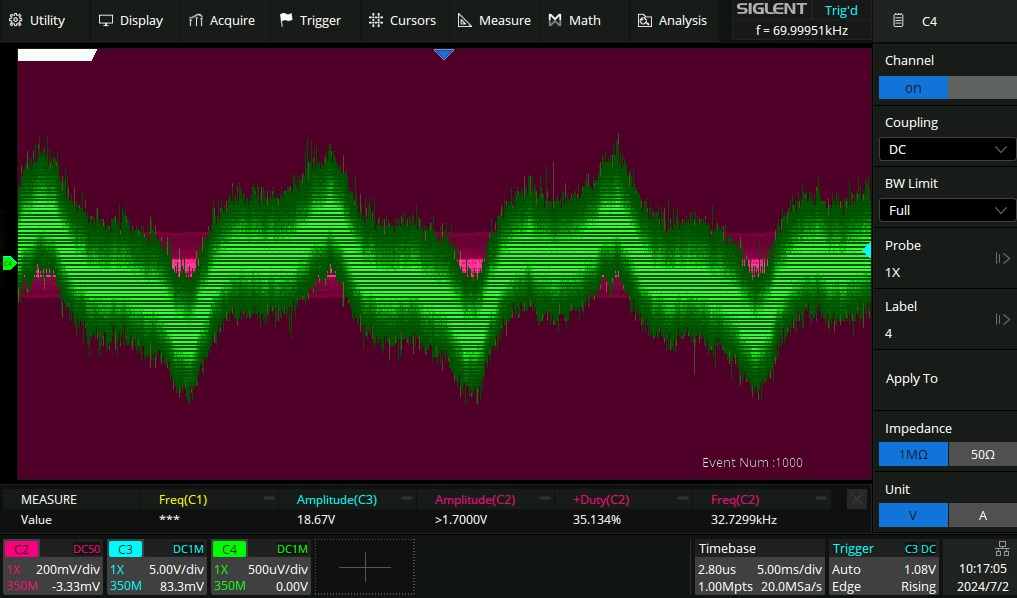
here is what the magnetometer looks like detecting a 1KHz sine wave:

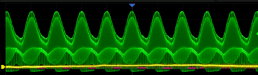
The magnetometer is being driven at 70kHz.

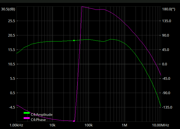
Bandpass filter

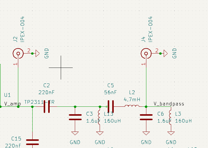
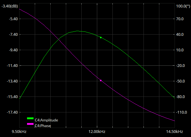
…Not great.

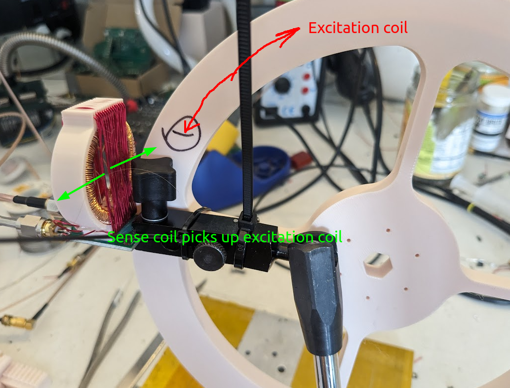
Using magnetometer to sense 11kHz magnetic field.

This is starting to get a bit tricky. I angled the magnetometer such that it was not receiving much magnetic field. Then I strapped a coil to it, and excited the coil at 11kHz (to fit inside the above bandpass later).

Setup:

There are three states here in the FFT plot:

No excitation, minimum magnetic field. This resulted in a peak at basically only 50kHz
No excitation, max magnetic field. Strong peaks at 100 and 200kHz appear in proportion to the strength of the field
Exciting with external field. Base 11kHz modulation appears, but there is a much stronger peak at 100kHz +/- 11kHz. This is also in direct proportion to the volts going into the coil, and is also independent of the external magnetic field.

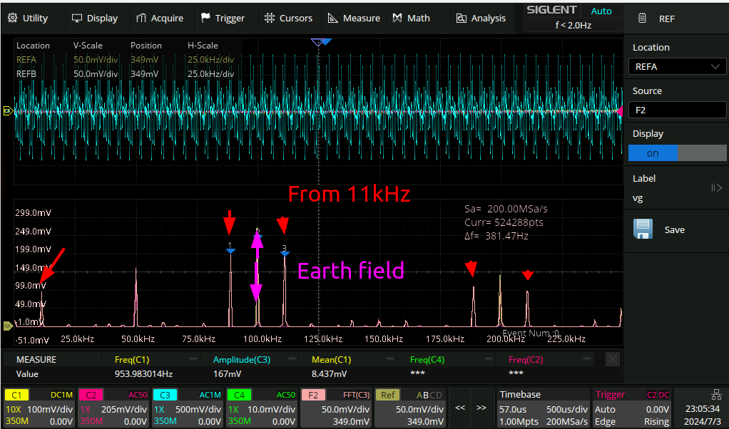
I had initially thought here that the strongest signal would show up at the base excitation freqency:

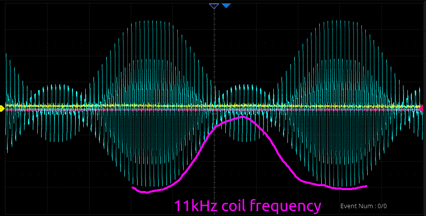
But from the above FFT it appears that this is not actually the case.

Measuring technique pivot.

I gave up on all of the above amplifiers and filters, I do not think they are necessary. Instead, I can just pull 100e6 samples off the scope and do an FFT to measure the power in the bands I care about directly. I think that’s a much better technique.

More current

I was barely receiving any signal at all from my magnetometer from my coil and I figure that was because I was driving it from my waveform generator rather than from a proper driver. So I resoldered the H bridge from the plasma toroid project and that pushed plenty of amps into the system. So many that I needed to put 3 5W 10R resistors in parallel so as not to hit the undervoltage lockout of the LMG chip. But after that it was fine.

Measuring the current

I can’t look at the high side of the coil and use the 50R impedance of the AWG to calculate the current going into this thing any more, since this is my setup now:

So I need another way to measure the current. I don’t have any current sense resistors (4 1.1R 0603 resistors in parallel blew up real quick) but I do have a stainless steel PCB stencil, so I chopped some of that and used it as a current sense resistor:

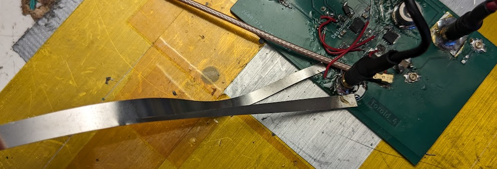
You may be wondering how one solders to stainless steel. It is in fact trivial with the tremendous flux that I was gifted. Naturally the label corroded off quite quickly and so I don’t know what brand it is precisely, but it is inside a secondary containment container with “STAY BRITE” on it.

Anyway the above current sense resistor is about 0.286 Ohms apparently.

This will be required later as the coil itself has some frequency response and so you can’t just assume the applied voltage translates to a current directly.

Analog current

Now I have things set up reasonably well I need to generate a signal at many different frequencies from my coil and measure it with the fluxgate magnetometer to prove this whole thing out. But the output of the above H bridge is always a square wave and so there will be all kinds of harmonics all over the place. I don’t want to deal with that, I want to measure one and only one frequency at a time!

No problem though, I will use the inductor in my coil like a motor winding and drive it like a BLDC sin drive! Here is the waveform snipped (ChatGPT was useless for this, ugh):

def generate_pwm_signal(N):
    window_size = 100
    out = np.ones(N)
    out_window = out[0:window_size * (N // window_size)].reshape((-1, window_size))
    subsize = out_window.shape[0]
 
    x = np.linspace(0, 2 * np.pi, subsize)
    sin = np.sin(x)
    sin_norm = (sin - np.min(sin)) / (np.max(sin) - np.min(sin))
    sin_norm = sin_norm * 0.8 + 0.2
 
    out_window[:] = np.linspace(0, 1, window_size).reshape((1, -1)) < sin_norm.reshape((-1, 1))
    remainder = N - subsize * window_size
    if remainder > 0:
        out[-remainder // 2:] = 1
    return out

This can then get uploaded to the scope. This results in the following current plot:

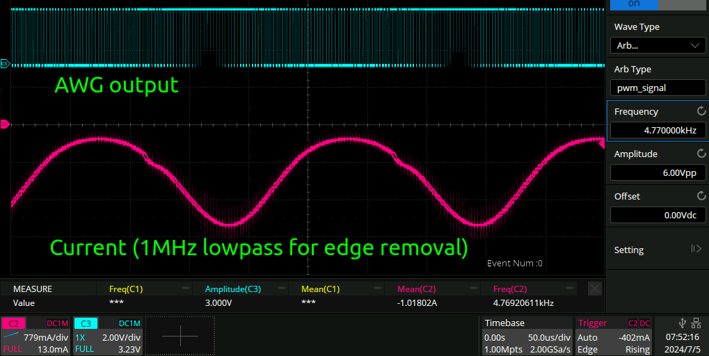
Which doesn’t look too bad. It didn’t replicate the low end very well so I had to do the sin = sin*0.8 + 0.2 above. I also had to make a tradeoff with the waveform output sample rate vs number of samples in the AWG sent to the scope, since the AWG uses the same csv file (it only takes csv files over usb stick) and just plays it back faster or slower. So above a certain waveform repetition rate it goes over the AWG sample rate and the whole thing falls apart. I could transfer a new csv file per frequency but pls, that ain’t gonna happen. The above waveform has 8192 samples and that allows it to go between 1 and 15kHz.

Now we are ready to make some measurements!

Measurement setup

The measurement setup looks like this:

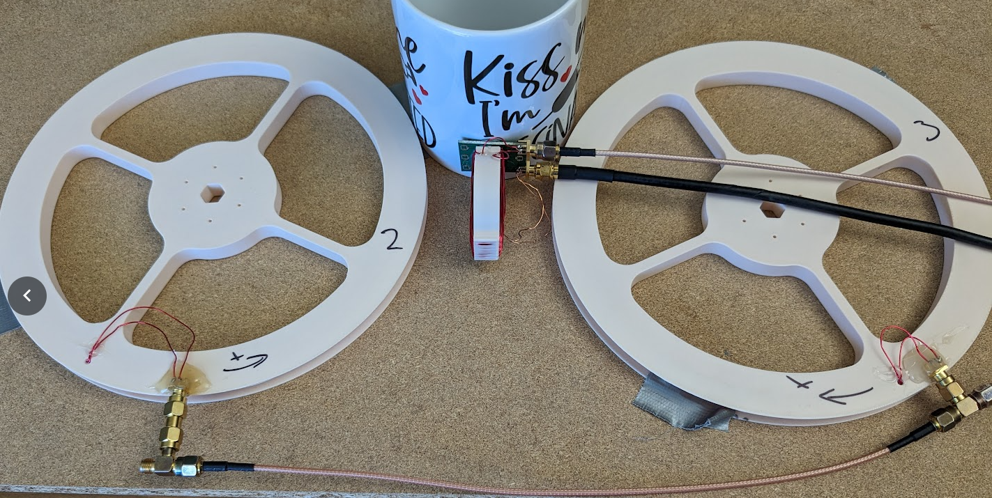
The idea here is that the two coils on either side are wound with the opposite circularity coil, and then placed in parallel. Per my previous simulations (and common sense) this means that there is a null in the middle where the magnetometer can be placed. The idea here is that it is similar to the double D coil setup that many other metal detectors use. The magnetometer is placed so that it is sensitive to fields in the vertical direction. There is a significant earth component in that direction too, but according to the above FFT measurements this should not affect things.

The magnetometer is hot glued to a mug so I can slide it around and get it into the right position. I do this in the time domain by just lookint at the scope and adjusting things so the persistence view shows that the amplitude is no longer being modulated. Interestingly it is not possible to zero out the field when the magnetometer is rotated 90 degrees so the donut is facing more towards the camera in the above pic (but is still vertical). I guess it’s just too wide and either side of the toroid is affected differently.

Test objects

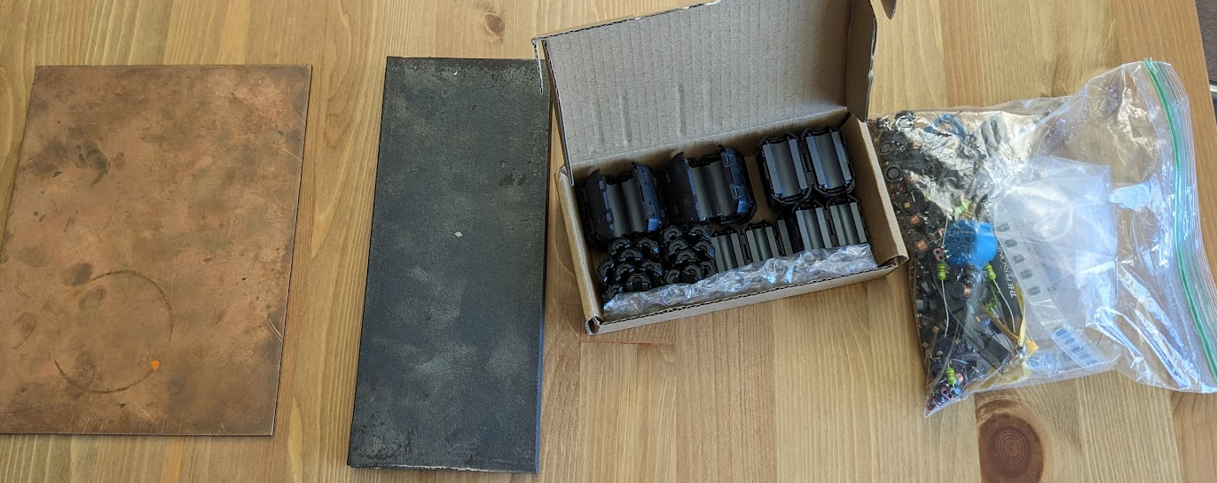
Here are the test objects with which to make measurements. You will notice they are not exactly subtle targets. This setup is very insensitive. The point here though is to see how things change over frequency, not the absolute level. I shall wave my hands and say that the setup is poorly optimised overall and surely if I built it for real I could make it much more sensitive.

Measurement technique (Siglent SCPI commands are garbage)

The siglent scope that I have has 500Mpoints of memory. So the idea here was to use a computer to control the AWG of the scope to output the right sin drive PWM wave for the given measurement frequency. Then I could pull the waveform down to the computer again using SCPI However:

When using the SCPI command C{channel}:WF? DAT2 to pull waveforms off the scope, if you specify any more than 10e6 waveforms you just get back 10e6, even though the acquisition may have been for 100e6 samples.
Therefore you have to save data to a USB in a mysterious binary format if you want all your samples
None of the USB SCPI commands work, they all timeout
There are no SCPI commands for controlling the waveform generator it seems So to take a given measurement the workflow was to do the following manually:

Change the AWG frequency
Press ‘acquire’ and wait ~15a
Save the waveform (100e6 points at 10MSa/s)
Run a script to record the metadata (which target, which frequency etc.) Then in post I use the date modified timestamp on the oscilloscope file with the timestamp of when I ran the above script to associate the waveform data with the metadata. Disgusting.

Also, the setup is quite insensitive, so I had to place the copper/ferrite targets directly on the coil right next to the mug to get a signal. This makes me a bit worried as perhaps I am blocking the field from one of the coils rather than introducing a new field from either eddy currents or distortions.

Measurement results

I measured three things:

Copper plate
Ferrite
Nothing, but with the magnetometer offset from center slightly to get some signal For each of these things I measured 1-15kHz in 1kHz steps which was incredibly tedious. Each measurement point here from the scopes points of view is essentially a 4*100e6 array of samples. That represents a full 10 seconds of data so there is quite a lot of averaging happening.

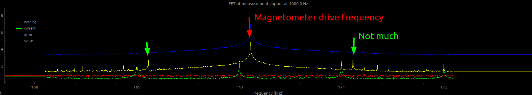
I drove the magnetometer drive coil at 170’112Hz. I chose this rando frequency so it wouldn’t be a multiple of any of the modulation frequencies.

Another thing of note here is that the ferrite caused a significant DC change in the measured magnetic field, which is what you would expect for something ferromagnetic. To convince myself that there would be no eddy currents here I measured the resistance of the ferrite material and it is indeed an open circuit.

Time series

Not much interesting here but I shall show it for completeness

Frequency 0 → modulation kHz

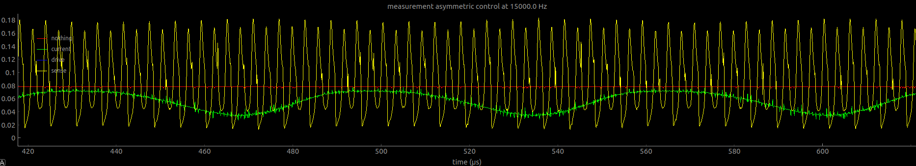
The below spectrograms have all been averaged with a 2Hz wide filter, as otherwise they were incredibly noisy and full of spikes.

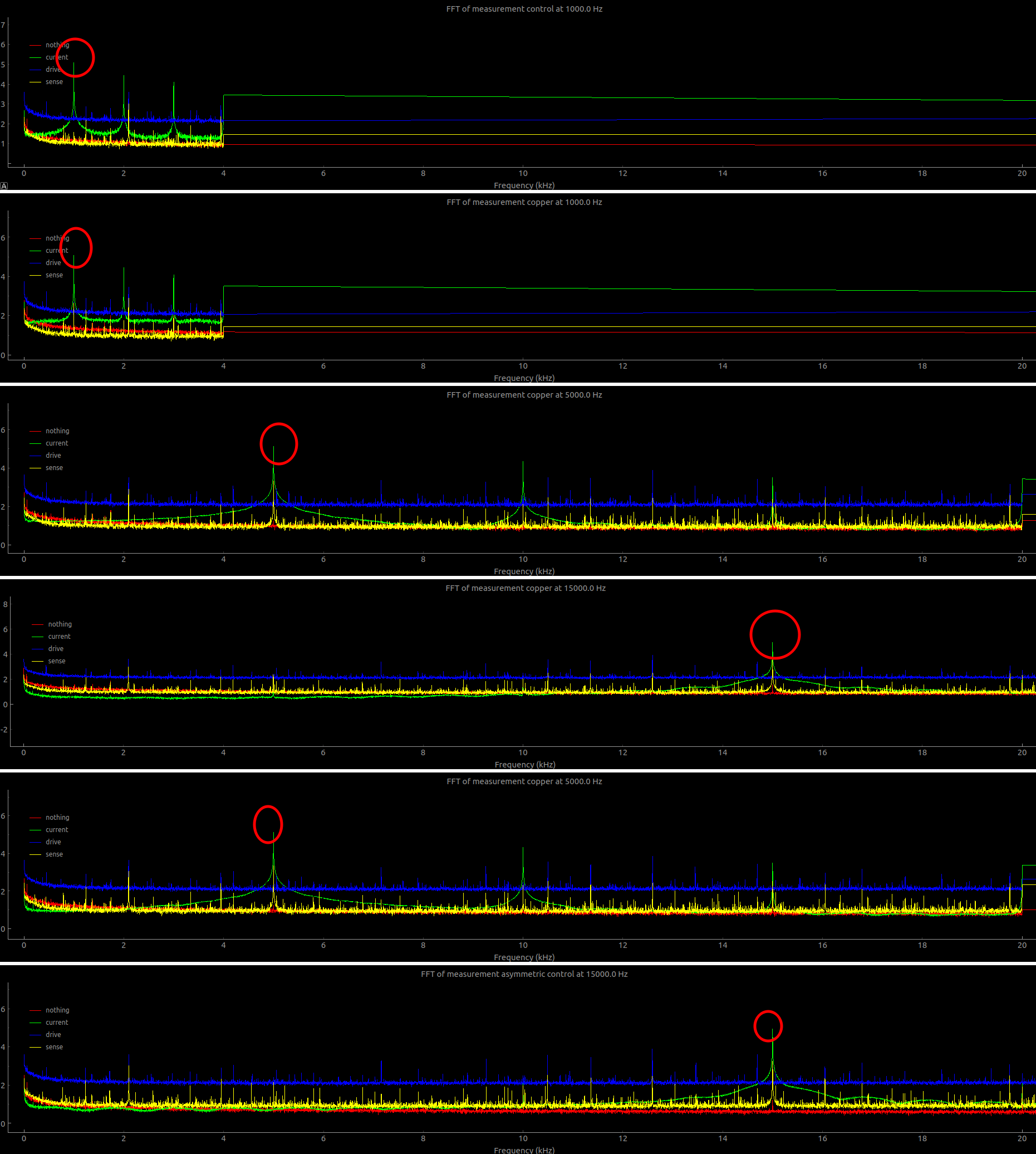
The circled parts of the green trace above are the measured currents being used to modulate the two coils. Since this is AM modulation, this apparently should show up on either side of the main drive. The reason some of the measurement above is chopped out is for plot rendering performance.

Around magnetometer drive frequency

Around 2 * magnetometer drive frequency

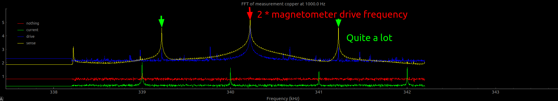
The reason that the signal from the magnetometer shows up at 2x the frequency is because fluxgate magnetometers get a pulse every time the winding magnetises and demagnetises, so you get 2 pulses per period.

Cooked measurements

So I get one of the above spectrograms per measurement. The next thing to do is to extract out what the magnetometer is actually measuring. To do this I just placed a 10Hz wide bandpass filter around +/- 2x the modulation frequency and called that the ‘sense’ measurement, since it is the sense winding of the magnetometer. I also put a 10Hz wide band around the measured current going through the coil, since it is possible that this also changes as a function of frequency

Volts as a function of frequency

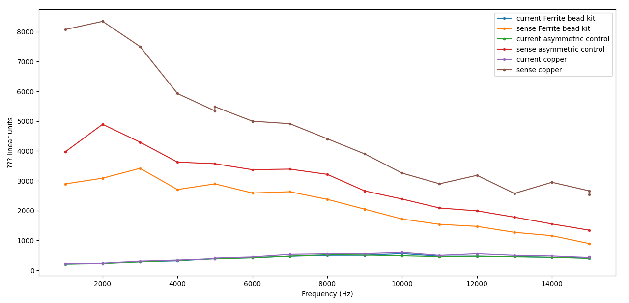
So we can see here first off that the current going through the modulation coil is pretty flat. Also all of the measurements including the control slope down with frequency. So I guess the magnetometer doesn’t have such a flat frequency response after all.

You can also see that for the copper I took a measurement twice at 5 and 15kHz. They were both very consistent so I think this measurement has pretty good snr.

Signal as a function of frequency

Here I have divided the signal for each of the actual measured objects by the signal when there was no object, the control. The absolute signal level for the control is arbitrary and was just set by how much off-center I placed the magnetometer when making the measurement. The idea was to directly measure the magnetometers bandwidth so it could be controlled for. Since the current measurement looks flat I didn’t bother controlling for that.

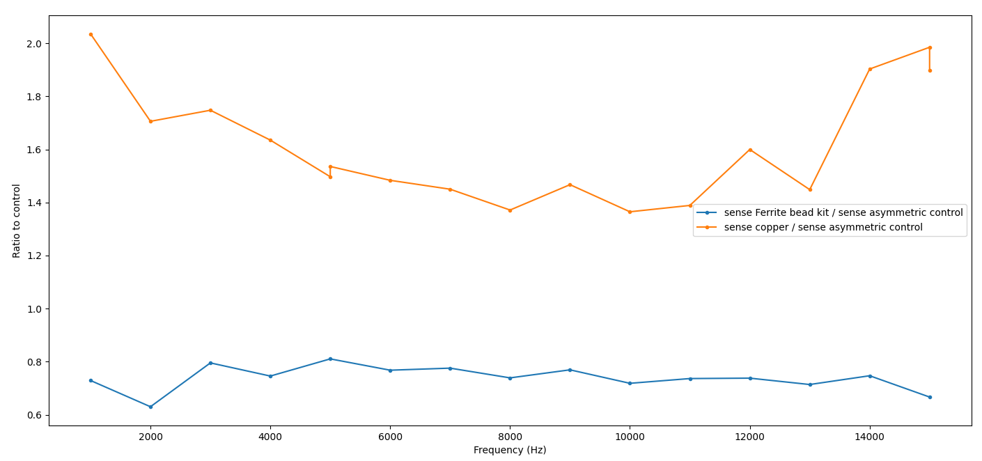
…And it looks like both of them are completely flat. That is exceedingly disappointing, I was hoping the slope would look like this:

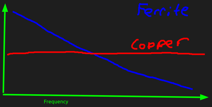
Hopeful reasons for this result

It is possible though that this is still the case. It could be for two reasons that I can think of

The measurement did not go low enough in frequency
Ferrite and copper do have quite a different response vs frequency but that was not what I was observing. Because the setup was so insensitive I had to place both the ferrite and the copper plate right inside basically touching the magnetic field. This could have set up an imbalance from the beginning that was much larger than the actual signal I wanted to measure.

Quartz 4

Explorer

20240701 Fluxgate magnetometer