I’ve always wondered why when people are looking for rocks, mineral deposits and so on they don’t just stick some sound transducers in the ground, blast out broadband noise, receive said noise, then calculate the 3D volume of the ground from that?
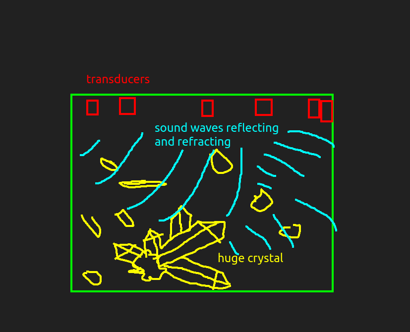
This is technically possible. It is called ‘Full wave inversion’. It has been done for some 2D mediums, but ChatGPT informs me it has not yet been done for 3D volumes of any significant size (say 512 elements cubed).
Problem
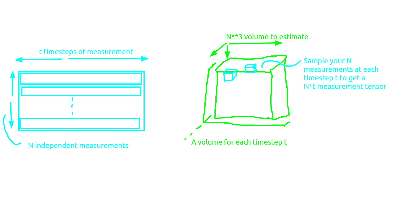
To be precise, if you have N transducers placed on the ground, t observations, and have a volume that is L voxels on a side, then the problem you need to solve is somehow converting the tensors N * t -> L**3. The term of art here is ‘Full waveform Inversion’.
 ** Actually I mean a
 L**3 volume in this diagram.
Quantity of data
The naive way to do this is to have a model of the propogations of waves through the ground. Then for a given timestep t, given your L**3 ground volume you can calculate a new L**3 ground volume at timestep t+1. For a volume of size 512 it will probably take at least 10e3 timesteps to simulate the whole thing. So to after simulating your 10e3 timesteps you have 1.3e12 voxels. Since the t*N**3 tensor is the whole state of the system let’s call it S.
Backpropogate to success
If you start with a totally homogenous medium and propogate it forward in time for your t timesteps, you can derive your N*t vector trivially by just measuring the voxels your detector was in. measurements = S[:, M_x, M_y, M_z where M_... are the coordinates of each measurement device. Then you can get the error in your system by just subtracting these modelled measurements from your actual measurements which if you recall are one of the inputs to the system.
Now you have an error, you can backpropogate it! This will adjust the medium to better fit the observations. Once the medium is adjusted to best fit the observations, it is the correct medium!
Memory requirements
Naively though, you need to back propogate through your whole state S. That requires many terabytes of memory, and so while it is just barely feasible with a modern GPU cluster, surely it is possible to do better. Recall that what we are actually trying to calculate here has only 512**3 elements, or 130e6. In addition to this the physics of wave propogation are relatively simple, and the actual volume you are trying to estimate is probably fairly compressible (each voxel is not independent of all other voxels, there is some structure). Surely estimating a space with size 130e6 does not require 1.3e12 elements of memory!
Reducing the memory requirements.
Save less
When each timestep is simulated, it produces a whole volume of size L**3. But we only observe N measurements from it. Maybe if I just save those N measurements, then I can do the update in-place and don’t need to save the full state S? I feel like this might make it a lot harder to train though since lots of the information has been straight up thrown away, rather than compressed. ChatGPT agrees with me, but it isn’t trustworthy on this kind of stuff. Worth some experiments.
Latent space
Other people have apparently gone the route of performing the simulation in some latent space. Nobody has gotten far enough as getting it to work for a full volume though.
Most trivial experiments
Here the goal is for the net to learn the contents of the simulation. The simulation has occurred on a 2D grid, and within that there are a set of ‘sensors’ that measure what is happening at each timestep. By having a lot of ‘sensors’ all over the grid, and feeding the input coordinates of the sensors into the net, the net can learn the entire output waveform for any given sensor because it has baked in the contents of the simulation.
This is what the last timestep of the simulation looks like, you can see there are lots of waves bouncing around and so on:
def generate_training_data(n_cells: int, n_sensors: int):
    """Return (sensor_positions[int 2×N], sensor_data[float N×T], true_density[H×W])."""
    domain = Domain((n_cells, n_cells), (0.1e-3, 0.1e-3))

    density = np.ones(domain.N) * 1000.0
    density[30:50, 30:50] = 2300.0
    density = FourierSeries(np.expand_dims(density, -1), domain)
    medium = Medium(domain=domain, sound_speed=1500.0, density=density)
    time_axis = TimeAxis.from_medium(medium, cfl=0.3)

    sensor_positions = np.random.randint(int(n_cells * 0.1), int(n_cells * 0.9), size=(2, n_sensors))
    sensor_positions[:, 0] = np.array([n_cells // 2, n_cells // 2])  # centre pixel
    sensors = Sensors(sensor_positions)

    p0 = circ_mask(domain.N, 3, (n_cells // 2, n_cells // 2))
    p0 = FourierSeries(jnp.expand_dims(p0, -1), domain)

    @jit
    def simulator(c_, p0_):
        med = Medium(domain=domain, sound_speed=1500.0, density=c_)
        return simulate_wave_propagation(med, time_axis, p0=p0_, sensors=sensors)

    t0 = time.time()
    sensor_data = simulator(density, p0)          # [N×T×1] JAX array
    print(f"forward simulation: {time.time() - t0:.2f} s")

    sensor_data = np.asarray(sensor_data.squeeze().T)  # → [N, T] NumPy
    return sensor_positions, sensor_data, density.params.squeeze()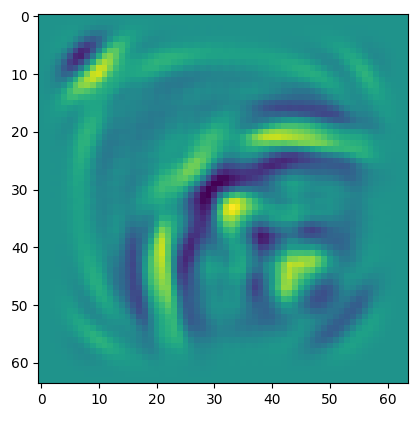
Training runs
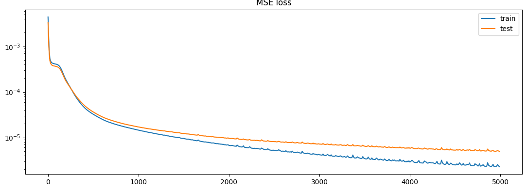
4 layers, 128 hidden dim:
- step 4990: train 2.2889e-06 | test 4.9705e-06
 4 layers, 64 hidden dim:
- step 4990: train 7.4923e-06 | test 1.0594e-05
4 layers, 256 hidden dim: step 4990: train 7.3234e-07 | test 3.5591e-06
None of the results here are particularly good. In particular, Just averaging the 4 adjacent cells produces a much lower loss than what the net can do. This says that there isn’t any interpolation going on, and the net has just gone off on the wrong track.
RBF embedding
This is apparently a better embedding sometimes:
import numpy as np
import matplotlib.pyplot as plt

def rbf_embedding(coords, centers, sigma):
    """
    coords  : (N, 2) array of input points normalised to [0,1]^2
    centers : (D, 2) array of RBF centres
    sigma   : float, shared width of the Gaussians
    returns : (N, D) embedding matrix
    """
    diff = coords[:, None, :] - centers[None, :, :]   # (N, D, 2)
    dist2 = np.sum(diff**2, axis=-1)                  # (N, D)
    return np.exp(-dist2 / (2.0 * sigma**2))          # (N, D)

nx, ny = 100, 100
xs = np.linspace(0.0, 1.0, nx)
ys = np.linspace(0.0, 1.0, ny)
grid_x, grid_y = np.meshgrid(xs, ys)
coords = np.stack([grid_x.ravel(), grid_y.ravel()], axis=-1)   # (N, 2)

dim = 3
cx, cy = np.linspace(0.0, 1.0, dim), np.linspace(0.0, 1.0, dim)
centers = np.stack(np.meshgrid(cx, cy), axis=-1).reshape(-1, 2)   # (dim^2, 2)
sigma = 0.15                                                      # width
X_nn = rbf_embedding(coords, centers, sigma)   # <‑‑ tensor for the NN

fig, axes = plt.subplots(dim, dim, figsize=(7, 7))
for i, ax in enumerate(axes.flat):
    im = X_nn[:, i].reshape(ny, nx)
    ax.imshow(im, origin="lower", extent=[0, 1, 0, 1])
    ax.set_xticks([])
    ax.set_yticks([])
    ax.set_title(f"Basis {i}")

fig.suptitle(f"First {dim**2} Gaussian RBF basis functions", y=0.92)
plt.tight_layout()
plt.show()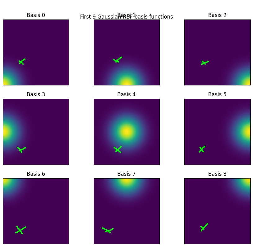
So here the coordinate marked with an X, which is about [0.2, 0.2] would be embedded with a number something like [0.01, 0.01, 0 | 0.01, 0.1, 0, | 0, 0, 0 ].
Sinusoidal embedding vs RBF embedding
Sinusoidal
step 4990: train 7.6137e-06 | test 2.1500e-05
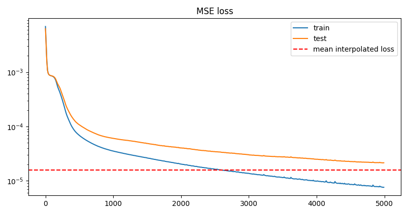
RBF embedding
step 4990: train 5.9338e-06 | test 1.0699e-05
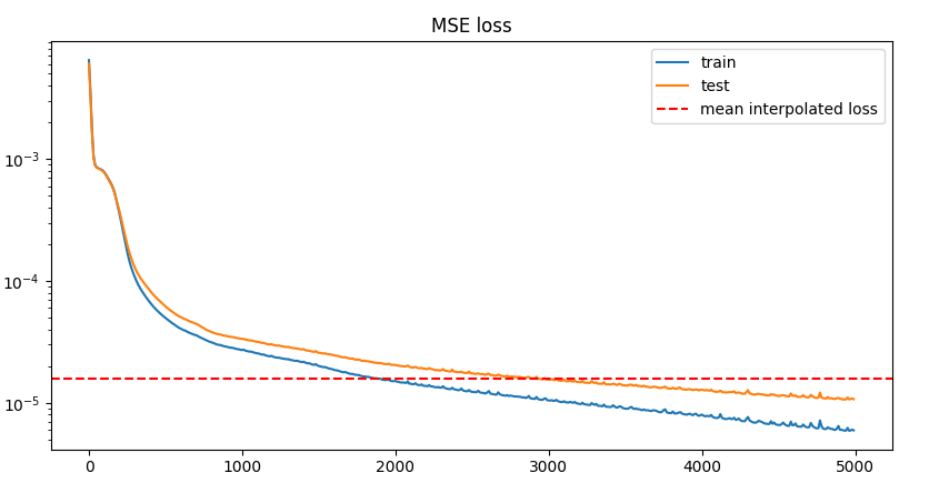
So RBF it is.
Full wave inversion
Now that that seems to mostly kinda work, time to move on. There is a good tutorial on doing full wave inversion for a 2D environment.
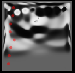
Here is the 2D field of sound speeds that should be recovered:
Here it is being recovered:
The scattered elements here are randomly scattered sensors. If there are N sensors, the simulation ‘data’ is a set of N simulations where each of the N sensors sends out a signal to the other (N-1) sensors in turn. So there are a total of (N-1)**2 time series waveforms of data.
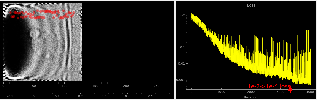
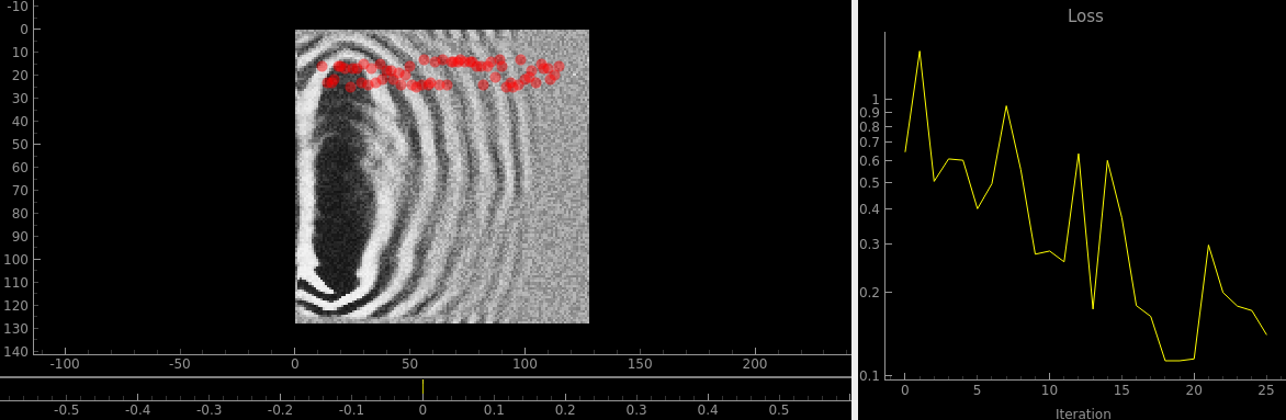
Sensors at the top
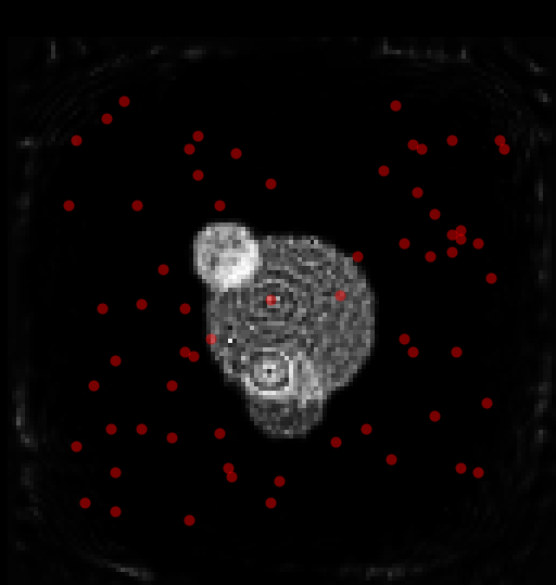
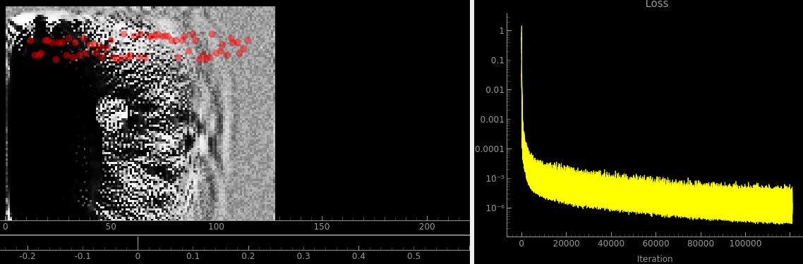
Of course, for this application, the sensors will be on the surface of the ground and the whole volume of the ground will need to be imaged. This is what things look like if you spread the sensors out near the top:
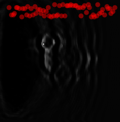
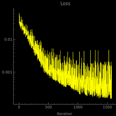
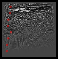
The loss curve is not exactly pretty though, and gives some hope that it could work better:
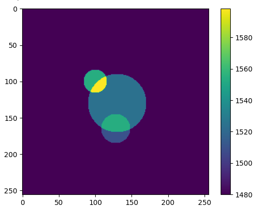
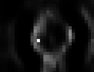
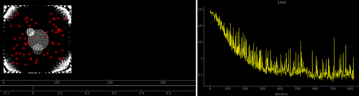
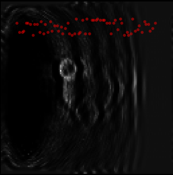
Interestingly much of the density seems to be concentrated into a single pixel for some reason:
Random initialization
You can actually just barely see the correct answer hiding here. but again the loss function is horrific. The loss is bouncing up and down by 3 OOM per iteration, surely it doesn’t have to do that. And it’s not like the image on the left changes in appearance a lot between iterations.
Better fitness function
Since from above we can see that very small changes in the predictions result in very large changes in the loss, we need a better fitness function. Since the current one is based on subtracting time series signals maybe if we just FFT things before doing the subtraction like so:
    def loss_func(params, src_idx):
        sos_fs = get_sound_speed(params, mask)           # FourierSeries
        pred    = sim_fn(sos_fs, src_idx)
        target  = p_data[src_idx]
        # return jnp.mean((hilbert_transf(pred) - hilbert_transf(target)) ** 2)
        pred_cook =   jnp.abs(jnp.fft.fft(hilbert_transf(pred)))
        target_cook = jnp.abs(jnp.fft.fft(hilbert_transf(target)))
        return jnp.mean((pred_cook - target_cook) ** 2)
Things will be better. The tutorial already started with the hilbert function, which was a new function that I didn’t know about and is fantastic. Here’s what the error looks like with the FFT loss function:
Compared to regular least squares:
Looks pretty similar, have to say. But they both look better than the one above. I think maybe what’s going on here is that (once again) the net has to predict something across a large dynamic range. This simulation is subject to the inverse square law just like the N body gravitational simulation i.e. when a sensor is placed close to an emitter the signal is absolutely huge compared to when it’s far away, but the far away signals are very important too!
The actual predicted outputs are a [64, 777] array and so chatGPT suggested normalising on a per row basis. I ran this overnight and got this result:
Aside from being the best result so far (you can clearly see the circle near the middle) the fitness function also has the least noise, though it still varies by an OOM. I don’t think this is a great solution still though since:
- The amplitude information between sensors is now lost
- The fitness function is still jumping around a whole bunch.
- This huge hole opened up on the left hand side in the first couple of iterations, and it hasn’t gone away over the whole training process.
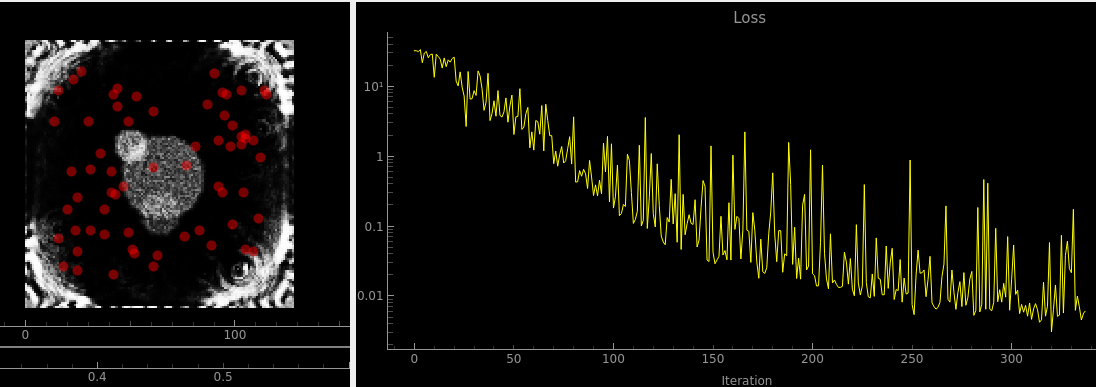
Bad-ish initialization
The field is initialized to be uniform random noise. But gradually over the first 25 iterations or so, this pattern reliably appears:
With some variations, this pattern is more or less the same when:
- varying the seed for generating the sensor locations
- Swapping out various fitness functions.
- Changing the initial conditions from random noise to a uniform field Initializing the field to a significantly negative value, so that all the corrections are in a positive direction seems to make things a bit better, in the sense that you can start to see the outline of the original velocity field, but the same massive ripples are still present:
And you can see that the stats continue to be bad - the loss is jumping around by orders of magnitude once again:
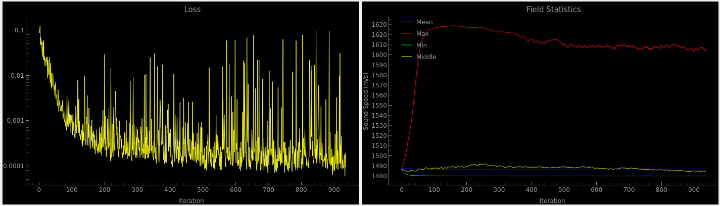
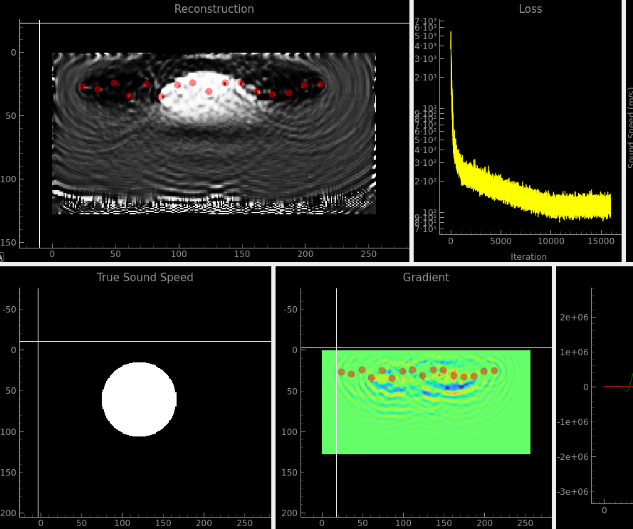
12 hour run
Here is an extremely weird plot of the loss and the speed of sound in the center of the grid:
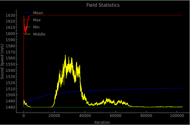
Who knows what this means..
A clue
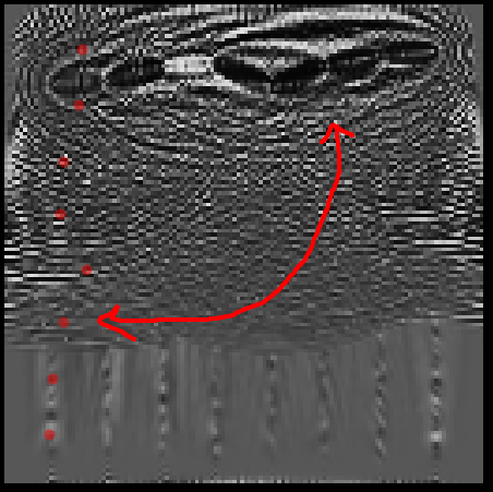
Throughout this whole sim there has been a persistent big ‘hole’ on the left hand side which I had been chalking up to Bad initialization. But just now I added a gradient plot so I can see how thing are being updated, and this is what came up:
Gradient
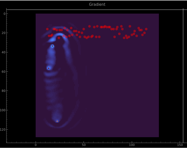
The three dots there have a magnitude 100x larger than any other pixels! That’s it! Now it is a question of finding out how they arose.
Things that don’t work to remove the gradient singularities
- Larger batch size
- Using a large batch size with a median. The actual singularities are removed, but the ripples from them are not.
- Doing all calculations in float64 - to try to rule out numerical precision issues
- Moving the circles in the sound speed grid around
- Transposing the x and y positions of the sensors transposes the positions of the singularities.
- Increasing the duration of the simulation. The current duration is set by the amount of time taken for a signal to propogate from one end of the grid to the other. Since this problem involves scattering, I thought the required time might be longer. But no, you get the exact same singularities pretty much.
Things that have some effect
- Source frequency. The tutorial had 1e6. This is what 1e7 looks like:

And 1e5:
If you squint it kind of looks like there is a transpose-like pattern showing up in the gradients.
Changing the source waveform to a nasty nasty chirp with unterminated ends gives this:
So from this we can say that the problem is related to the source signal.
The same signal with not only a higher source frequency but also a shorter duration chirp:
There is obviously something going on with the transpose of the source locations.
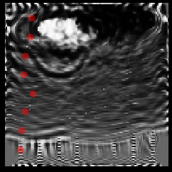
Inverting the signal
Regular, before inversion
After inversion
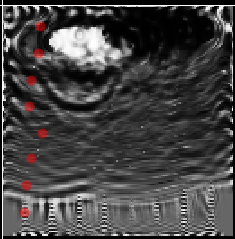
… Well that’s exactly the same. I was hoping that the white/black in the top would be flipped, so that the two could be averaged out to get a correct result.
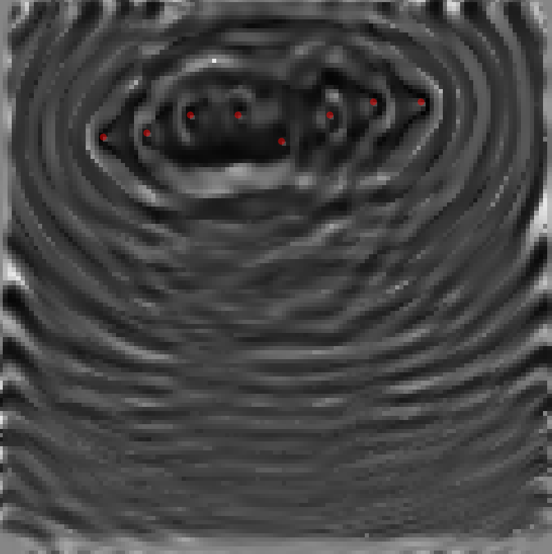
Transpose
… of course, the x/y of the image coordinate system was different to that of the sensor positions, so the discontinuities are on top of the sensor locations.
I also discovered a bunch of bugs in the loss function whereby the hilbert transform was being performed over the wrong axis of the measurement matrix. After fixing that, and after zeroing out the ith-to-ith sensor measurement (i.e. the sensor measuring itself) I get this:
Which is not that much better, really.
2:1 aspect ratio long run
From the above, and moving the sensor locations 20 units away from the edge due to the 20 wide boundary condition, the sensors didn’t really have a good angular spread anymore which I figure is necessary to get good diversity of angles looking at what we want to reconstruct. So I changed it to a 2:1 aspect ratio:
This seems to have done a kind of OK job, but clearly the ripples are still causing a lot of problems and it completely loses the bottom of the circle. You can also see in the gradient view that most of the effort is going towards the close-in stuff.